1. Reference problem#
1.1. 3D geometry#
The structure is a straight parallelepiped with a square base. The dimensions of the bar (see []) are: \(\mathit{LX}\mathrm{=}\mathrm{5m}\), \(\mathit{LY}\mathrm{=}\mathrm{5m}\) and \(\mathit{LZ}\mathrm{=}\mathrm{25m}\).
The interface is introduced by level sets directly into the command file using the DEFI_FISS_XFEM [U4.82.08] operator. The interface is present in the middle of the structure through its representation by a level set \(\text{LSN}\) (see []) equation:
\(\text{LSN}\text{(pour le plan de l'interface) :}Z-\frac{\mathrm{LZ}}{2}\)
Figure 1.1-b
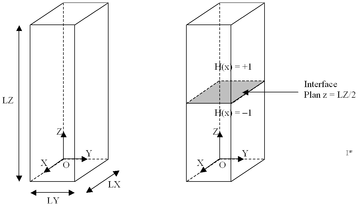
Figure 1.1-a : Bar geometry and interface position
1.2. 2D geometry#
The structure is a rectangle. The dimensions of the bar (see []) are: \(\text{LX}\mathrm{=}\mathrm{1m}\), \(\text{LY}\mathrm{=}\mathrm{5m}\).
The interface is introduced by a level set function directly into the command file using the DEFI_FISS_XFEM [U4.82.08] operator. The interface is present in the middle of the structure through its representation by a level set \(\text{LSN}\) (see []) equation:
\(\text{LSN}\text{(pour le plan de l'interface) :}Y-\frac{\mathrm{LY}}{2}\)
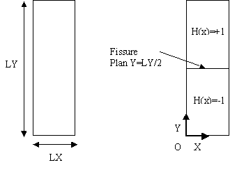
Figure 1.2-a : Plate geometry and interface position
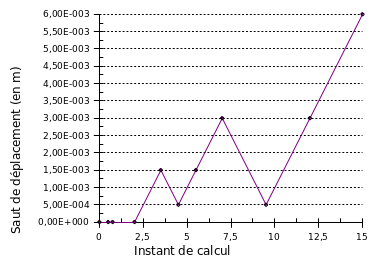
Figure 1.2-b : Evolution of the displacement jump imposed by piloting as a function of the calculation instant
1.3. Material properties#
Young’s module: |
\(\text{E = 0,5.E6Pa}\) |
Poisson’s ratio: |
\(\nu \mathrm{=}\mathrm{0,0}\) |
The presence of a cohesive law at the interface is specified using the keyword RELATION =” CZM_EXP_REG “when defining the contact zone (command DEFI_CONTACT, keyword factor ZONE). The cohesive law then implemented has parameters \({G}_{c},{\sigma }_{c}\) and \({\kappa }_{0}\) as parameters, and is explained in detail in the documentation [R7.02.11]
Tenacity: |
\({\text{G}}_{\text{c}}\mathrm{=}\text{900 N/m}\) |
(keyword: GC) |
Critical stress at rupture: |
\({\sigma }_{c}\mathrm{=}\text{1,1.E6 Pa}\) |
(keyword: SIGM_C) |
Energy regulation parameter: |
\({\kappa }_{0}\mathrm{=}\mathrm{1,0E-3}\) |
(keyword PENA_ADHERENCE) |
Note:
Material data is, of course, not intended to represent a particular material. They are only intended for numerical validation tests.
1.4. Boundary conditions and loads#
1.4.1. Enriched degrees of freedom and boundary conditions#
Recall that the displacement under \(X-\mathrm{FEM}\) is the sum of a continuous displacement and a discontinuous displacement. In the case of an interface, with no cracks, the approximation of the displacement is written as follows:
\({u}^{h}(x)=\sum _{i\in {N}_{n}(x)}{a}_{i}{\phi }_{i}(x)+\sum _{j\in {N}_{n}(x)\cap K}{b}_{j}{\phi }_{j}(x)H(\mathrm{lsn}(x))\)
Where:
\({a}_{i}\) and \({b}_{i}\) are the degrees of freedom of movement at node \(i\),
\({\phi }_{i}\) the shape functions associated with node \(i\),
\({N}_{n}(x)\) is the set of nodes whose support contains the point \(x\),
\(K\) is the set of knots whose support is entirely cut by the crack,
\(H(x)\) is the generalized Heaviside function defined by \(H(x)=\{\begin{array}{}-1\text{si}x<0\\ +1\text{si}x\ge 0\end{array}\),
\(\mathrm{lsn}(x)\) is the normal level-set value at point \(x\).
For more details, refer to reference documentation \(X-\mathrm{FEM}\) [R7.02.12].
It is therefore possible to want to impose limit conditions on the total displacement (or physical displacement), on its continuous component or on its discontinuous component. First, we will give various useful relationships between this physical displacement and the degrees of freedom existing in Code_Aster.
Let’s take the example shown: an edge of any \(\mathrm{2D}\) mesh crossed by an interface:
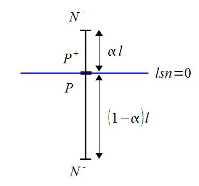
Figure 1.4.1-1: Edge intersected by an interface
Let’s call \({P}^{\text{+}}\) and \({P}^{\text{-}}\) the geometric points belonging to the segment and located respectively just below and above the level set and consider vertical displacements without losing generality. We have:
\(\mathrm{\{}\begin{array}{c}\mathit{DY}({N}^{\text{+}})\mathrm{=}{a}_{y}^{\text{+}}+{b}_{y}^{\text{+}}\\ \mathit{DY}({N}^{\text{-}})\mathrm{=}{a}_{y}^{\text{-}}\mathrm{-}{b}_{y}^{\text{-}}\\ \mathit{DY}({P}^{\text{+}})\mathrm{=}\alpha ({a}_{y}^{\text{+}}+{b}_{y}^{\text{+}})+(1\mathrm{-}\alpha )({a}_{y}^{\text{-}}+{b}_{y}^{\text{-}})\\ \mathit{DY}({P}^{\text{-}})\mathrm{=}\alpha ({a}_{y}^{\text{+}}\mathrm{-}{b}_{y}^{\text{+}})+(1\mathrm{-}\alpha )({a}_{y}^{\text{-}}\mathrm{-}{b}_{y}^{\text{-}})\end{array}\)
From this we can derive the expression for the jump in displacement for the edge:
\(\mathrm{〚}\mathit{DY}\mathrm{〛}\mathrm{=}\mathit{DY}({P}^{\text{+}})\mathrm{-}\mathit{DY}({P}^{\text{-}})\mathrm{=}\alpha {b}_{y}^{\text{+}}+(1\mathrm{-}\alpha ){b}_{y}^{\text{-}}\)
1.4.2. Loading#
In \(I\) mode, the nodes on the lower face of the bar are embedded and a vertical displacement is imposed on those on the upper face, as explained in the figure.
In opening mode \(\mathrm{II}\), the nodes located under the level set are embedded, and a vertical movement \(\mathit{DY}\) (\(\mathit{DZ}\) in \(\mathrm{3D}\)) of \(\mathrm{1,0E-13}\) is imposed on all nodes located above the level set. In this way, the contact indicator is null and void at the interface level. We also impose pure shear at the level of the cohesive zone, which, taking into account the notations in the figure, is equivalent to imposing for each intersected edge:
\(\mathrm{\{}\begin{array}{c}\mathit{DX}({P}^{\text{-}})\mathrm{=}\mathit{DX}({N}^{\text{-}})\mathrm{=}0\\ \mathit{DX}({P}^{\text{+}})\mathrm{=}\mathit{DX}({N}^{\text{+}})\end{array}\)


Figure 1.4.2-1: Load applied, in mode \(I\) and in mode \(\mathrm{II}\)
We see that this requires imposing connections between degrees of freedom on both sides of edge \(i\) that depend on the coefficient \(\alpha\). In order not to unnecessarily burden the command file, we will only test meshes in \(\mathrm{II}\) mode for which:
or all the intersected edges are intersected in their middle, that is to say that for each \(\alpha \mathrm{=}\mathrm{0,5}\)
or the interface is compliant, i.e. \(\alpha \mathrm{=}1\)
In the first case, where all the edges are intersected in their middle, we ensure the nullity of the contact indicator by imposing \(\mathit{H1Y}\mathrm{=}5.E\mathrm{-}14\) on all the node ends of the edges intersected by the interface. With respect to shear, we need to impose the relationships:
\(\mathrm{\{}\begin{array}{c}\mathit{DX}({P}^{\text{-}})\mathrm{=}\mathit{DX}({N}^{\text{-}})\mathrm{\iff }\frac{{a}_{x}^{\text{+}}\mathrm{-}{b}_{x}^{\text{+}}}{2}+\frac{{a}_{x}^{\text{-}}\mathrm{-}{b}_{x}^{\text{-}}}{2}\mathrm{=}{a}_{x}^{\text{-}}\mathrm{-}{b}_{x}^{\text{-}}\mathrm{=}0\\ \mathit{DX}({P}^{\text{+}})\mathrm{=}\mathit{DX}({N}^{\text{+}})\mathrm{\iff }\frac{{a}_{x}^{\text{+}}+{b}_{x}^{\text{+}}}{2}+\frac{{a}_{x}^{\text{-}}+{b}_{x}^{\text{-}}}{2}\mathrm{=}{a}_{x}^{\text{+}}+{b}_{x}^{\text{+}}\end{array}\)
We then see that if we impose the \({a}_{x}^{\text{+}}\mathrm{=}{b}_{x}^{\text{+}}\) relationship then \(\mathit{DX}({P}^{\text{-}})\mathrm{=}0\).
If we then impose the \({b}_{x}^{\text{+}}\mathrm{=}{b}_{x}^{\text{-}}\) relationship, we also have \(\mathit{DX}({P}^{\text{+}})\mathrm{=}\mathit{DX}({N}^{\text{+}})\).
In the second case, with an interface conforming to the mesh, the jump is represented by the Heaviside degree of freedom at the point combined with the interface and we must therefore impose \(\mathit{H1Y}\mathrm{=}1.E\mathrm{-}13\) on the nodes combined with the interface. As far as shear is concerned, if \({N}^{\text{-}}\) corresponds to the point coinciding with the \({P}^{\text{-}}\) interface, we must impose:
\(\mathrm{\{}\begin{array}{c}\mathit{DX}({P}^{\text{-}})\mathrm{=}{a}_{x}^{\text{-}}\mathrm{-}{b}_{x}^{\text{-}}\mathrm{=}0\\ \mathit{DX}({P}^{\text{+}})\mathrm{=}\mathit{DX}({N}^{\text{+}})\mathrm{\iff }{a}_{x}^{\text{-}}+{b}_{x}^{\text{-}}\mathrm{=}{a}_{x}^{\text{+}}\end{array}\)
We then see that if we impose the \({a}_{x}^{\text{-}}\mathrm{=}{b}_{x}^{\text{-}}\) relationship then \(\mathit{DX}({N}^{\text{-}})\mathrm{=}\mathit{DX}({P}^{\text{-}})\mathrm{=}0\).
If we then impose the \({a}_{x}^{\text{-}}\mathrm{=}\frac{{a}_{x}^{\text{+}}}{2}\) relationship, we also have \(\mathit{DX}({P}^{\text{+}})\mathrm{=}\mathit{DX}({N}^{\text{+}})\).
These two relationships are imposed for all the nodes in relation to the meshes crossed by the interface.
It should be noted that, in the command file, the syntax for imposing these different degrees of freedom differs between operators. The factor keyword DDL_IMPO of the AFFE_CHAR_MECA operator makes it possible to impose total displacement (or physical displacement) using the keywords DX, DY, and DZ, as well as the discontinuous degrees of freedom \({b}_{i}\) using the keywords H1X, H1Y, and H1Z. On the other hand, the keyword factor LIAISON_GROUP makes it possible to control the continuous degrees of freedom \({a}_{i}\) thanks to the keywords DX, DY, and DZ (and not the total displacement) as well as the discontinuous degrees of freedom \({b}_{i}\) thanks to the keywords H1X, H1Y, and H1Z.
1.5. Load control#
For mode \(I\), the control is performed on the vertical movement jump. The vertical displacement \(\mathrm{DY}\) (\(\mathrm{DZ}\) in \(\mathrm{3D}\)) imposed on the nodes of the upper face of the bar is then unitary. The real intensity of the movement of these nodes is therefore known during the calculation by means of the parameter ETA_PILOTAGE. One of the SAUT_IMPO or SAUT_LONG_ARC controls implemented specially for \(\mathrm{XFEM}\) is used, on the normal component \(\mathrm{H1Y}\) (\(\mathrm{H1Z}\) in \(\mathrm{3D}\)), corresponding to \({b}_{y}\) (\({b}_{z}\) in \(\mathrm{3D}\)) with the notations taken above, for all the edges intersected by the interface.
For mode \(\mathrm{II}\), the control is performed on the horizontal movement jump. The control is then carried out in an identical manner to mode \(I\), but on the tangential component \(\mathit{H1X}\).
Finally, for each of the opening modes, the controls used make it possible to explore all the phases of the law of behavior: elastic linear load, damage and discharge.
FIGS. 1 and 5 represent the evolution of the displacement jump as a function of the calculation instant. In order to perform discharges, several times of calculation (keyword reuse) are performed to make it possible to change the value of the coefficient \({c}_{\mathrm{mult}}\) (keyword COEF_MULT) making it possible to define the value of the increment of the displacement jump \(\Delta {\delta }_{i}\) to be imposed for a time step \(\Delta t\) via the control equation. Since the problem is uniform, this relationship is written in a simple way for SAUT_IMPO and SAUT_LONG_ARC: \(\Delta {\delta }_{i}{c}_{\mathit{mult}}\mathrm{=}\Delta t\). Type PRED_ELAS control is not yet tested for this case because it would require a feedback giving the possibility of driving in a landfill, discussed in [R5.03.80], with this type of piloting.
Charging takes place in ten phases, thanks to ten successive calls to STAT_NON_LINE:
Final calculation instant |
Phase |
Final move jump (in \(m\) ) |
C mult DDL_IMPO LONG_ARC |
C mult PRED_ELAS |
0.5 |
Start of initial elastic load |
2.73E-7 |
1.833350000E+06 |
1.500013700E+03 |
0.75 |
Initial elastic discharge |
1,36E-7 |
-1.833350000E+06 |
-1.500013700E+03 |
2 |
End of initial elastic load |
8,18E-7 |
1.833350000E+06 |
1.500013700E+03 |
3 |
Damage 1 |
1.50E-3 |
1.000545747E+03 |
1.001000991E+00 |
3.5 |
||||
8.001501926E-01 |
||||
4 |
Elastic discharge 1 |
5,00E-4 |
-1.000000000E+03 |
-8.501501892E-01 |
4.5 |
||||
-1.285714290E+00 |
||||
5 |
Elastic load 1 |
1.50E-3 |
1.000000000E+03 |
1.285714286E+00 |
5.5 |
||||
8.001501912E-01 |
||||
7 |
Damage 2 |
3,00E-3 |
1.000000000E+03 |
2.089908926E+00 |
9 |
Elastic discharge 2 |
5,00E-4 |
-1.000000000E+03 |
-1.641475407E+00 |
9.5 |
||||
-1.285714290E+00 |
||||
10 |
Elastic load 2 |
3,00E-3 |
1.000000000E+03 |
1.285714286E+00 |
12 |
||||
1.441475409E+00 |
||||
15 |
Damage 3 |
6,00E-3 |
1.000000000E+03 |
4.179817852E+00 |
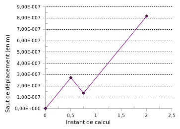
Figure 1.5-1 : Evolution of the displacement jump imposed by piloting up to calculation time 2.
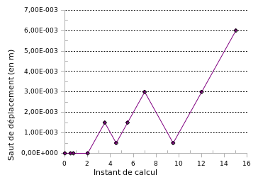
Figure 1.5-2 : Evolution of the displacement jump imposed by piloting as a function of the moment of calculation.