2. Reference solution#
The reference solutions for the three pipe geometries are obtained by elastoplastic modeling with isotropic work hardening and Von Mises criterion with Code_Aster in axisymmetric massive finite elements on a very refined quadratic mesh: 100 meshes in the thickness, cf. Modeling A. We can also compare the solutions with the results obtained in [bia1] _ and [bib2] _ with a mesh made with 10 quadratic axisymmetric finite elements and an elastoplastic calculation using isotropic work hardening and Von Mises criterion with Alibaba.
The equation of the radial static equilibrium of the pipe under internal and external pressures independent of \(z\), cf. é 3.3.1 of [bib3] _, leads to the expression of the mean circumferential stress in the thickness, regardless of the behavior of the material:
\(\overline{\sigma_{\theta\theta}}=\frac{N_{\theta\theta}}{h}=\frac{1}{h}\int_{R_i}^{R_e}\sigma_{\theta\theta}\left(r\right)dr=\frac{R_i+R_e}{2h}\left(p_i-p_e\right)- \frac{p_i+p_e}{2}\)
For paths 1 and 2, we describe the elastoplastic material with isotropic work hardening with the traction curve including a perfect plastic plate, see section Reference problem.
All the curves that represent the dependence of the fields in thickness are plotted with a dimensionless abscissa between 0, for the inner radius, and 1 for the outer radius.
For path 1 (cyclical internal and external pressures)
The radial displacement over time of the axisymmetric finite element modeling is plotted on the inner wall, on the outer wall, and on the middle sheet.
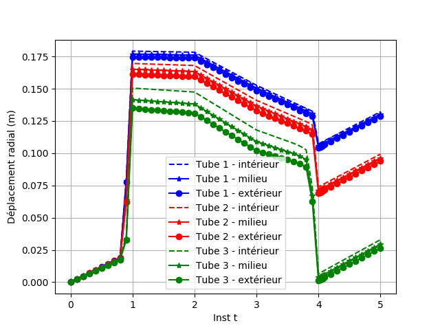
Fig. 2.1 Radial displacement#
The axial displacement over time of the axisymmetric finite element modeling is plotted on the middle sheet.
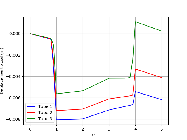
Fig. 2.2 Axial displacement#
The circumferential stresses in the wall at time 1 and at time 4, interpolated at the nodes of the mesh, are plotted from the values at the Gauss points.
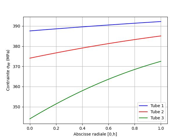
Fig. 2.3 Circumferential stresses at time 1#
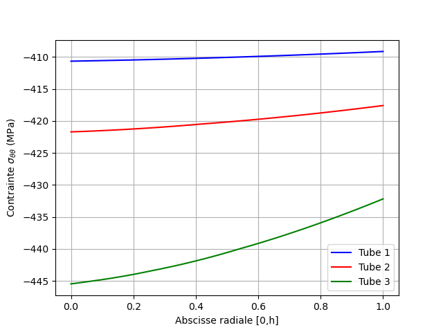
Fig. 2.4 Circumferential stresses at time 4#
The plastic deformations accumulated in the wall at instant 1 and at time 5, interpolated at the nodes of the mesh, are plotted from the values at the Gauss points.
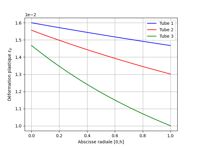
Fig. 2.5 Plastic deformation at instant 1#
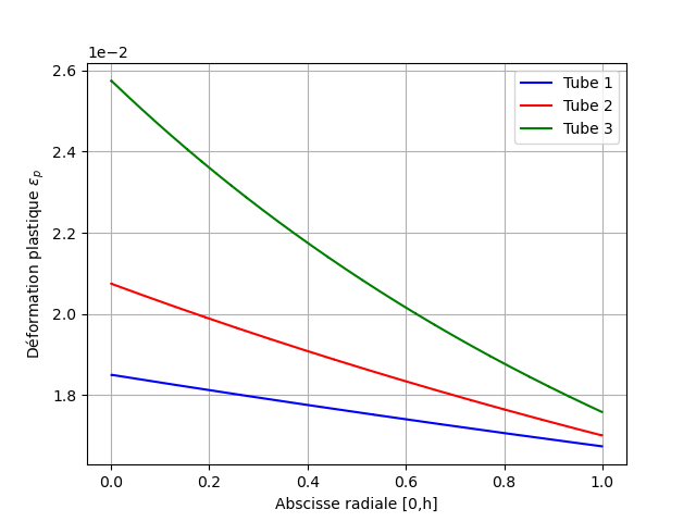
Fig. 2.6 Plastic deformation at instant 4#
For path 2 (monotonous internal pressure to ruin)
We recall the expression (obtained by R.Hill, cf. eq 8.7.9 of [bib3] _) for the ruin pressure in pure radial plastic flow of a plugged tube under internal pressure with Von Mises criterion:
\(p_{ruine}= \frac{2 \sigma_{y} \sqrt{3} }{3} ln \left( \frac{{R}_{e}}{{R}_{i}} \right)\)
Taking into account work hardening, we also find the approximate expression of the ruin pressure of a plugged tube which involves the average between the elastic limit (taken conventionally at 0.2% plastic deformation) and the plastic flow limit:
\(p_{ruine}^{éc}= \frac{ \left( \sigma _{y}+\sigma _{u}\right) \sqrt{3} } {3} ln \left( \frac{{R}_{e}}{{R}_{i}} \right)\)
With the data provided in Reference problem, we obtain the numerical values using numerical simulation using axisymmetric 2D finite elements for an unplugged tube:
Tube \(h/R\) |
\(p_{ruine}^{éc}\) (\(\mathit{MPa}\)) |
Dimensional pressure |
0.05 |
33.20 |
33.20 |
0.10 |
66.45 |
33.23 |
0.20 |
133.24 |
33.31 |
The radial displacement is plotted as a function of the internal pressure over time of the modeling in axisymmetric elements on the middle sheet. We forced uniformity in thickness
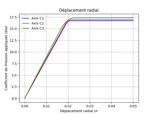
Fig. 2.7 Radial displacement#
The radial stresses in the wall at time 3 and at time 5, interpolated at the nodes of the mesh, are plotted from the values at the Gauss points.
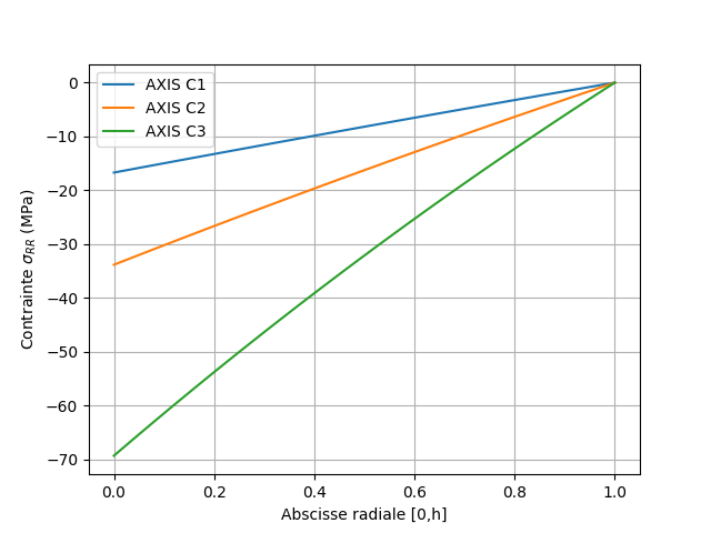
Fig. 2.8 Radial stresses at time 3#
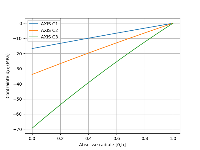
Fig. 2.9 Radial stresses at time 5#
The circumferential stresses in the wall at time 3 and at time 5, interpolated at the nodes of the mesh, are plotted from the values at the Gauss points.
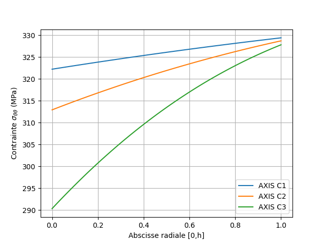
Fig. 2.10 Circumferential stresses at time 3#
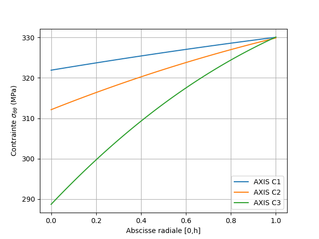
Fig. 2.11 Circumferential stresses at time 5#
The plastic deformations accumulated in the wall at time 3 and at time 5, interpolated at the nodes of the mesh, are plotted from the values at the Gauss points.
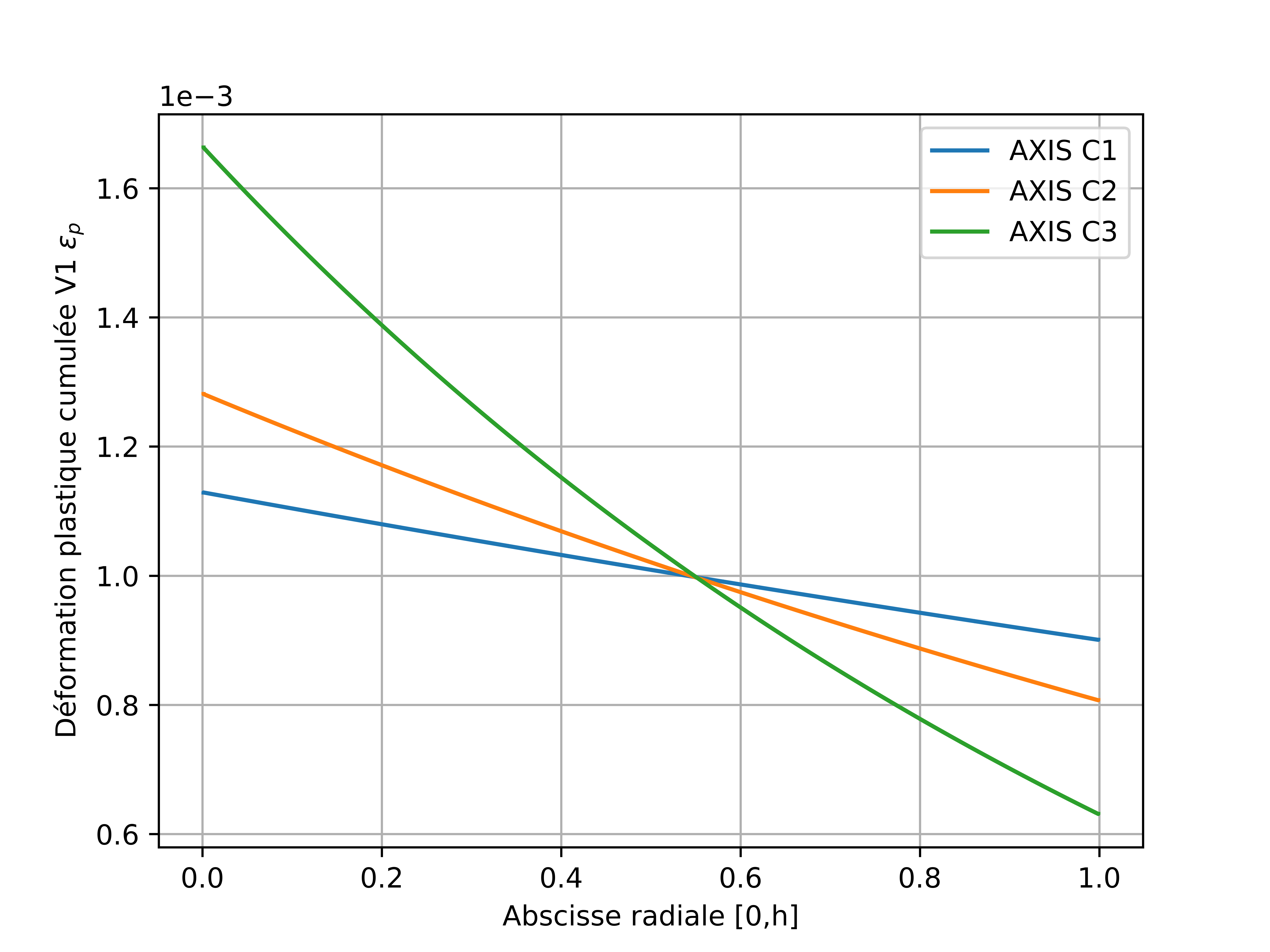
Fig. 2.12 Plastic deformation at instant 3#
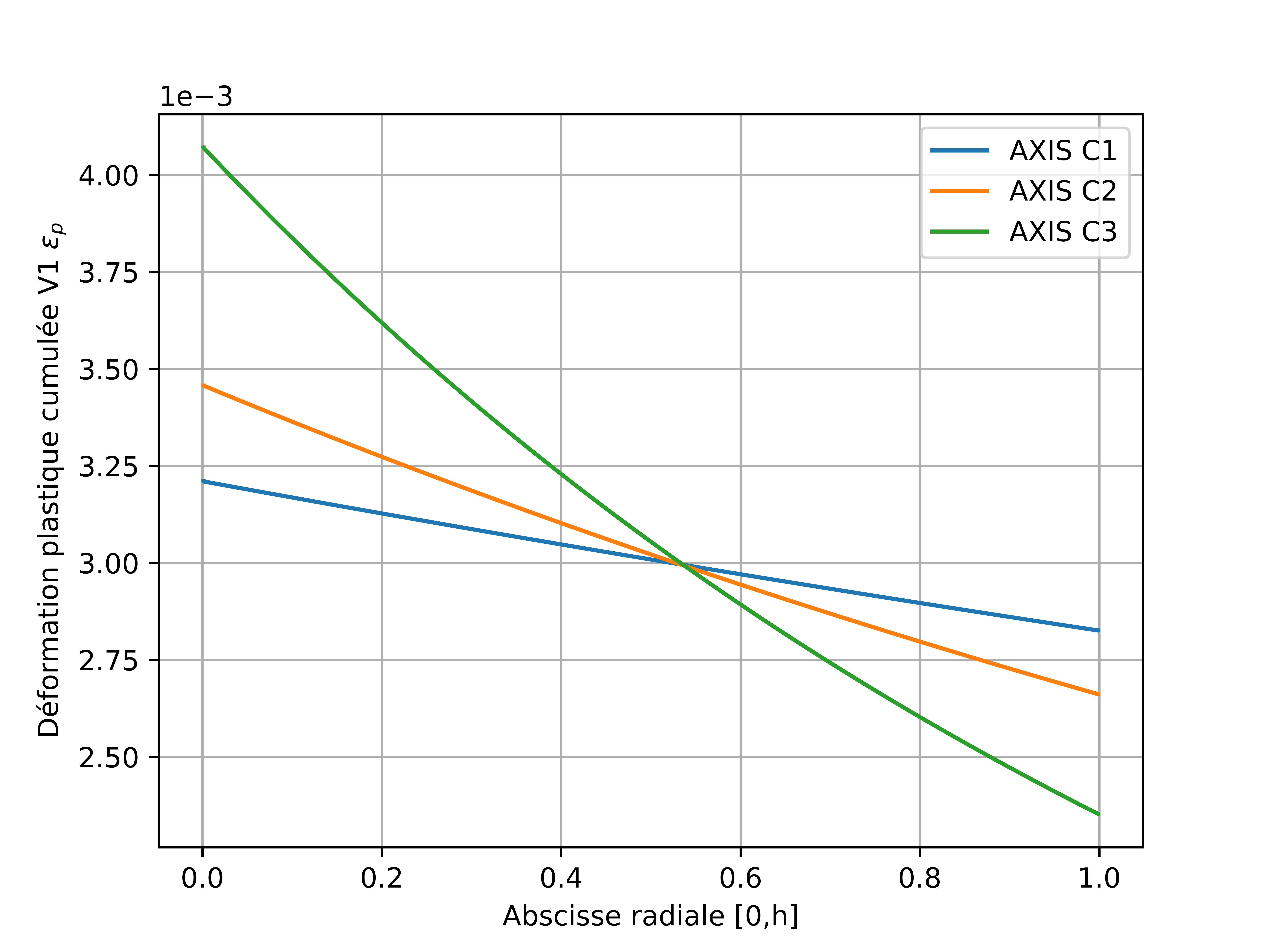
Fig. 2.13 Plastic deformation at instant 5#