3. Modeling A#
3.1. Characteristics of modeling#
DALLE
Y
A3
A4
A2
A1
LSYMY
LSYMX
LCONTX
LCONTY
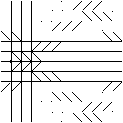
Q4GG modeling (TRIA3)
Boundary conditions:
. Side \(\mathrm{A2A4}\): \(\mathrm{DZ}=0\)
Symmetry conditions
. Side \(\mathrm{A1A2}\): \(\mathrm{DY}=\mathrm{DRX}=0\)
. Side \(\mathrm{A1A3}\): \(\mathit{DX}\mathrm{=}\mathit{DRY}\mathrm{=}0\)
X The slab is symmetric with respect to planes \((X\mathrm{=}0)\) and \((Y\mathrm{=}0)\), the calculations are carried out on a quarter of the slab.
3.2. Characteristics of the mesh#
Number of knots: 169
Number of meshes and type: 288 TRIA3
3.3. Tested sizes and results#
Identification |
Reference Type |
Reference |
Tolerance (%) |
\(\mathit{DZ}(\mathit{A1})\) |
“ANALYTIQUE” |
6,926.10-5 |
|
\(\mathit{MXX}(\mathit{A1})\) |
“ANALYTIQUE” |
1550 |
|
\(\mathit{MYY}(\mathit{A1})\) |
“ANALYTIQUE” |
1550 |
|
\(\mathit{KXX}(\mathit{A1})\) |
“ANALYTIQUE” |
2,193.10-4 |
|
\(\mathit{KYY}(\mathit{A1})\) |
“ANALYTIQUE” |
2,193.10-4 |
|
The quantities are expressed in the coordinate system defined by the nautical angles \(\alpha \mathrm{=}33°\) and \(\beta \mathrm{=}12°\)
Identification |
Reference Type |
Reference |
Tolerance |
\(\mathrm{DZ}(\mathrm{A1})\) |
“ANALYTIQUE” |
6,926.10-5 |
|
\(\mathit{MXX}(\mathit{A1})\) |
“ANALYTIQUE” |
1550.0 |
|
\(\mathit{MYY}(\mathit{A1})\) |
“ANALYTIQUE” |
1550.0 |
|
\(\mathit{MXY}(\mathit{A1})\) |
“ANALYTIQUE” |
||
\(\mathit{KXX}(\mathit{A1})\) |
“ANALYTIQUE” |
2.193 10-4 |
|
\(\mathit{KYY}(\mathit{A1})\) |
“ANALYTIQUE” |
2.193 10-4 |
|
\(\mathit{KXY}(\mathit{A1})\) |
“ANALYTIQUE” |
0.001 |
Identification |
Reference type |
Reference |
Tolerance% |
||
\(\mathit{MXX}\) |
\(\mathit{M266}\) |
\(\mathit{Point}3\) |
“NON_REGRESSION” |
1445.794 |
1.e-6 |
\(\mathit{MYY}\) |
\(\mathit{M266}\) |
\(\mathit{Point}3\) |
“NON_REGRESSION” |
1447.847 |
1.e-6 |
\(\mathit{MXY}\) |
\(\mathit{M266}\) |
\(\mathit{Point}3\) |
“NON_REGRESSION” |
0.526 |
1.e-6 |
\(\mathit{KXX}\) |
\(\mathit{M266}\) |
\(\mathit{Point}3\) |
“NON_REGRESSION” |
2.14096 10-4 |
1.e-6 |
\(\mathit{KYY}\) |
\(\mathit{M266}\) |
\(\mathit{Point}3\) |
“NON_REGRESSION” |
2.14565 10-4 |
1.e-6 |
\(\mathit{KXY}\) |
\(\mathit{M266}\) |
\(\mathit{Point}3\) |
“NON_REGRESSION” |
1.2018 10-7 |
1.e-6 |
3.4. notes#
The coefficients of the following elasticity matrices, used during the calculations, were calculated with \({\nu }_{b}=\mathrm{0,22}\):
Membrane elasticity matrix: \(\left[\begin{array}{ccc}4832& \mathrm{990,4}& 0\\ \mathrm{990,4}& 4832& 0\\ 0& 0& 1756\end{array}\right]{10}^{6}\text{N/m}\)
Flexural elasticity matrix: \(\left[\begin{array}{ccc}\mathrm{5,879}& \mathrm{1,188}& 0\\ \mathrm{1,188}& \mathrm{5,879}& 0\\ 0& 0& \mathrm{2,107}\end{array}\right]{10}^{6}\text{N/m}\)
To be certain of staying within the elastic domain, the elastic limits, expressed in the orthotropy coordinate system, are set arbitrarily to a very high value:
Elastic limits in positive flexure:
Direction x: \({1.10}^{10}\text{MNm/ml}\)
Direction y: \({1.10}^{10}\text{MNm/ml}\)
Elastic limits in negative flexure:
Direction x: \(\mathrm{-}{1.10}^{10}\text{MNm/ml}\)
Direction y: \(\mathrm{-}{1.10}^{10}\text{MNm/ml}\)
As the structure remains in the elastic domain, the kinematic recall coefficient (Prager constant) can take any value.