4. D modeling

4.1. Geometry and modeling

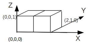
The mesh is composed of:

• 1 HEXA8sur mesh to which the 3D modeling is affected.

• 1 HEXA20sur mesh to which we assign the 3D modeling_ INTERFACE.

HEXA1	3D
HEXA2	3D_ INTERFACE

4.2. Orientation of the local coordinate system

In order to define the local coordinate system for these elements, the keyword factor MASSIF from the AFFE_CARA_ELEM operator is used (see U4.42.01).

Several ways of defining a local coordinate system are proposed, here we are testing ANGL_REP and the ANGL_AXE/ORIG_AXE couple.

The table above gives the orientations chosen for each element:

HEXA1	ANGL_REP	\((\mathrm{45.0,45}\mathrm{.0,90}.0)\)
HEXA2	ORIG_AXE/ANGL_AXE	\((\mathrm{100.0,0}\mathrm{.5,0}.5)\)/\((\mathrm{0.0,}-45.0)\)

4.3. Calculating local landmarks

The local landmarks are formed by the vectors \(x\), \(y\), and \(z\).

The values given in ANGL_REP define the following guidelines:

\(x=\left(\mathrm{0.5,0}\mathrm{.5,}-\frac{\sqrt{2}}{2}\right)\), \(y=\left(\mathrm{0.5,0}\mathrm{.5,}\frac{\sqrt{2}}{2}\right)\), and \(z=\left(\frac{\sqrt{2}}{2},-\frac{\sqrt{2}}{2},0\right)\).

The ANGL_AXE/ORIG_AXE pair is used in the case of a model with cylindrical geometry. They define an axis \({e}_{z}\) being the axis of the cylindrical coordinate system.

\(x\) corresponds to the vector \({e}_{z}\) of this cylindrical coordinate system, the reference point being the barycenter of the cell here \((1.5\mathrm{,0}.5\mathrm{,0}.5)\). \(y\) corresponds to the vector \(\mathrm{-}{e}_{\theta }\) and \(z\) to the vector \({e}_{r}\).

In this example \(x=\left(\frac{\sqrt{2}}{2},\mathrm{0,}\frac{\sqrt{2}}{2}\right)\), \(y\mathrm{=}(\mathrm{0,1}\mathrm{,0})\), and \(z=\left(\frac{-\sqrt{2}}{2},\mathrm{0,}\frac{\sqrt{2}}{2}\right)\).

4.4. Tested sizes

The tested results are shown in the following table:

MAILLE	Vector	Component	Reference Value	Tolerance
HEXA1	\(x\)	\(X\)		\(0.5\)	\(1.E\mathrm{-}8\)
HEXA1	\(x\)	\(Y\)		\(0.5\)	\(1.E\mathrm{-}8\)
HEXA1	\(x\)	\(Z\)		\(\mathrm{-}0.707106781186E0\)	\(1.E\mathrm{-}8\)
HEXA2	\(x\)	\(X\)		\(0.707106781186E0\)	\(1.E\mathrm{-}8\)
HEXA2	\(x\)	\(Y\)		\(0\)	\(1.E\mathrm{-}8\)
HEXA2	\(x\)	\(Z\)		\(0.707106781186E0\)	\(1.E\mathrm{-}8\)
HEXA1	\(y\)	\(X\)		\(0.5\)	\(1.E\mathrm{-}8\)
HEXA1	\(y\)	\(Y\)		\(0.5\)	\(1.E\mathrm{-}8\)
HEXA1	\(y\)	\(Z\)		\(0.707106781186E0\)	\(1.E\mathrm{-}8\)
HEXA2	\(y\)	\(Y\)		\(1\)	\(1.E\mathrm{-}8\)
HEXA2	\(z\)	\(X\)		\(\mathrm{-}0.707106781186E0\)	\(1.E\mathrm{-}8\)
HEXA2	\(z\)	\(Y\)		\(0\)	\(1.E\mathrm{-}8\)
HEXA2	\(z\)	\(Z\)		\(0.707106781186E0\)	\(1.E\mathrm{-}8\)