5. Post-treatments with ParAvis#
In this chapter, we discuss some specificities related to the visualization of sub-point fields using ParAvis. It is always possible to write the results as free text or as a table using the IMPR_RESU command in the result format or with the pair of commands CREA_TABLE, IMPR_TABLE.
5.1. Travel#
The post-processing of movements does not require a specific calculation. Output in MED format is done using the IMPR_RESU command.
The finite elements discussed in this modeling document are DKT and GRILLE_EXCENTRE. These elements have the degrees of freedom:
translation: DX, DY, DZ.
rotation: DRX, DRY, DRZ.
To facilitate the visualization of the deformed mesh in ParaVis (Warp By Vector filter), it is easier to specify only the degrees of freedom of movement, when creating the file:
IMPR_RESU (FORMAT = “MED”,
RESU =_F (RESULTAT = Rstnl, **** Rstnl, ,) , NOM_CMP =( “DX”, “DY”, “DZ”) ), )) ,) ** NOM_CHAM DEPL
)
5.2. Generalized efforts#
Post-processing the widespread efforts for DKT requires a specific calculation. The CALC_CHAMP command allows you to calculate the fields EFGE_ELGA, EFGE_ELNO which have the following components: NXX, NYY, NXY, MXX, MYY, MXY,, QX, QY.
The output in MED format is then done using the IMPR_RESU command.
Rstnl = CALC_CHAMP (refuse= Rstnl,
RESULTAT = Rstnl, CARA_ELEM = CareLem, TOUT = “OUI”,
CONTRAINTE =( “EFGE_ELNO”, )) **,
)
IMPR_RESU (FORMAT = “MED”,
RESU =_F (RESULTAT = Rstnl, Rstnl,, ), ** NOM_CHAM EFGE_ELNO
GROUP_MA =The mesh group, ,) **,
)
Note: GRILLE_EXCENTRE items currently do not have widespread efforts.
Note: It is not recommended to calculate the generalized efforts at the nodes EFGE_NOEU. The local references of the elements connected to the same node are « not necessarily » oriented in the same way, in this case the following alarm message is sent.
<A><UTILITAI_4> You requested the calculation of a field at the nodes on elements of structure. But the local landmarks of certain meshes surrounding nodes on which you requested the calculation are not compatible (At most, we have 90,0456 degrees of difference between the angles nautical boats defining these landmarks). Risk & Advice: You may get inconsistent results. It is therefore recommended to change the fields to a global coordinate system. useful for calculating the field at the nodes. This is an alarm. If you don’t understand the meaning of this alarm, you may get unexpected results! |
5.3. Constraints & internal variables at sub-points#
The post-processing of constraints or internal variables does not require a specific calculation. Output in MED format is done using the IMPR_RESU command. On the other hand, the elements used are elements with sub-points, so it is necessary when printing to specify the concept from the AFFE_CARA_ELEM command.
IMPR_RESU (FORMAT = “MED”,
RESU =_F (RESULTAT = Rstnl, CARA_ELEM =carelem,
GROUP_MA =( “Pb2 GToleBasSurf “, “Pb2”, “Pb2 GBeton “, “Pb2 NNp1”, “Pb2 NNp2 “, ),), **
NOM_CHAM =( “SIEF_ELGA”, )) **,
NOM_CMP =( “SIXX”, “SIYY”, “”, “”, “,” SIXY “, )) ,) **,
)
To visualize this field (which is in the sub-points) with ParAvis, you must choose the field and validate the choice with « Apply ».
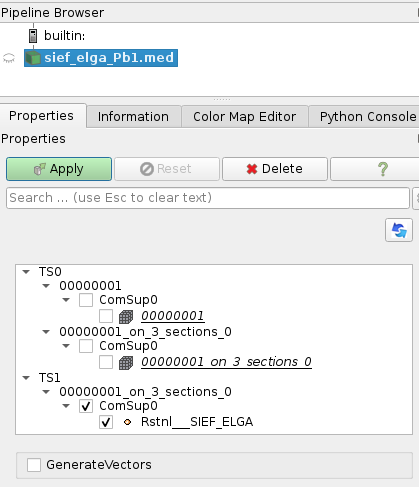
Then, you have to choose the component as well as the visualization at the gauss points
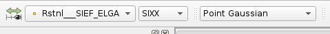
It may also be necessary to change the size of the « spheres » to visualize the field. This size should be given in the mesh unit. In the example, figure, the mesh is in meters, the size of the gauss points is 0.01m. The representation is made with spheres.
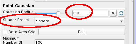
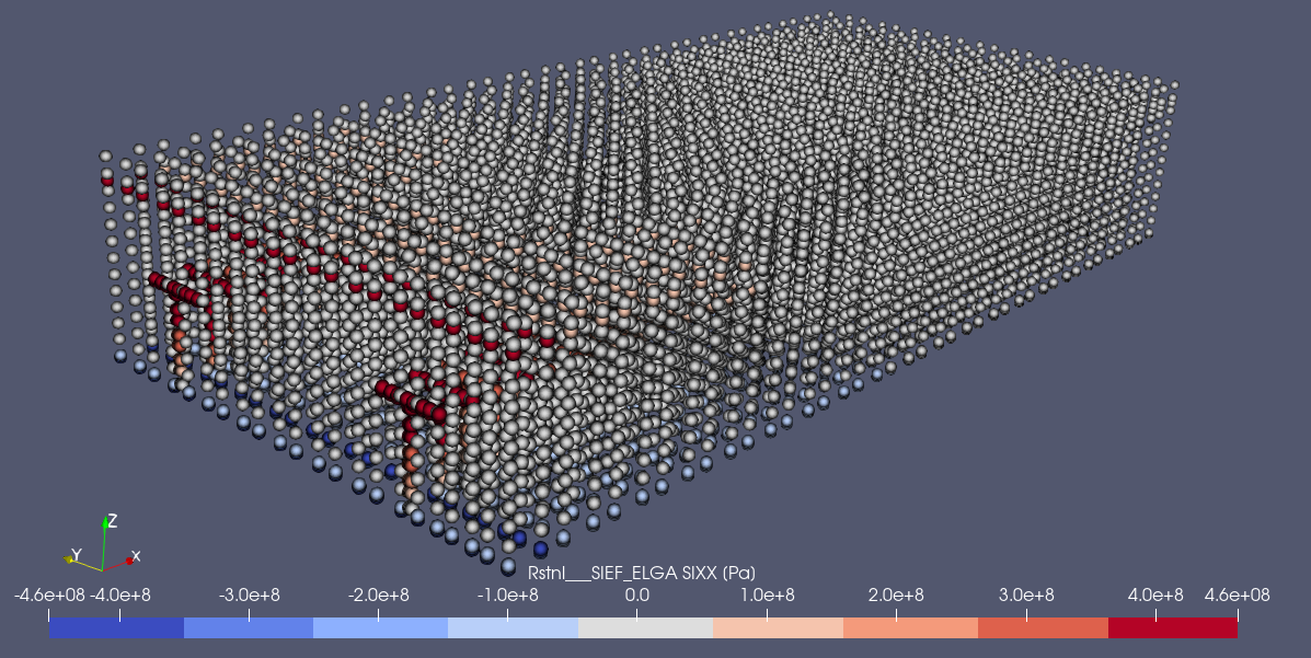
Figure 5.3-a : Visualization at sub-points, of the SIXX component of the constraint.
5.4. Fields at sub-points vs support elements#
Visualizing fields at sub-points (SIEF_ELGA, VARI_ELGA,…) can be quite difficult, due to the representation with « spheres » and their large number.
Code_aster allows you to extract components from fields to sub-points, and assign them to support elements (triangles, quadrangles).
The POST_CHAMP command with the MIN_MAX_SP factor keyword (SPpour subpoints) allows this extraction to be done. Several options are possible: “MAXI”, “MINI”, “”, “MAX_ABS”, “MINI_ABS”.
With this command and the keyword factor EXTR_COQUE, it is also possible to extract a field with all these components for a particular layer.
MaxVari = POST_CHAMP (
RESULTAT = Rstnl, GROUP_MA = List of mesh groups,
MIN_MAX_SP =(
_F (NOM_CHAM = “VARI_ELGA”, “,” “, ,) , TYPE_MAXI =**” MAXI_ABS “,** NUME_CHAM_RESU =**1**) ), NOM_CMP
_F (NOM_CHAM = “VARI_ELGA”, “,” “, ,) , TYPE_MAXI =**” MAXI_ABS “,** NUME_CHAM_RESU =**2**) ), NOM_CMP
),
)
IMPR_RESU (FORMAT = “MED”,
RESU =_F (RESULTAT = maxVari, IMPR_NOM_VARI = “NON”,
GROUP_MA = List of mesh groups,
NOM_CHAM =( “UT01_ELGA”, “UT02_ELGA”, “”, ), ), ), )) )) ,) **, NOM_CMP VAL
)
The figure shows the visualization of the field after using the POST_CHAMP command.
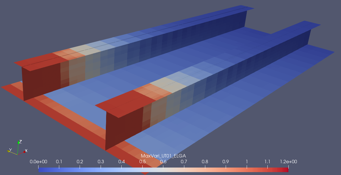
Figure 5.4-a : Representation of a component of a field at the sub-points, here VARI_ELGA, on the support elements.