5. How do I do a study?

This paragraph describes step by step how to use astk to conduct a study.

The study consists in calculating the response of a thin cylinder under hydrostatic pressure. The following elements are available:

The*Aster command file: forma00.comm

• The description of the geometry created with Salomé: forma00.datg

• The mesh size of the reservoir built by Salomé: forma00.mmed

The following results are produced:

• A result file in med format (travel fields,…): forma00.resu.med

• The classic Aster message and result files: forma00.mess and forma00.resu

In the example, we put all the files in the /home/tutorial directory.

The files in this example are available in the astest directory of your*Code_Aster* version.

Note:

In the case of a study with several command files, all the files must be of the « comm » type, associated with logical unit 1 and it is the order of appearance in the profile that determines the order of execution.

5.1. Creating the profile

We launch the interface which opens on a blank profile, or if astk is already launched, we choose*File/New* in the menu to create a new empty profile.

We go to the ETUDE tab.

5.2. Selecting files

5.2.1. Defining a base path

In tab ETUDE, we choose a base path to simplify file access.

We click on the icon

, we choose the /home/tutorial directory.

5.2.2. Add existing files

We add the command file by clicking on

, the file selection opens directly in the base path that we have just defined. All that remains is to select the file forma00.comm (double click or single click + ok), and the file appears in the list. Note that astk identifies the type of this file based on its « comm » extension, the logical unit number is set to 1, the « D » box (data) is checked.

The same is done for the mesh file in med format (forma00.mmed). astk recognizes the extension « mmed », the logical unit number is set to 20, the « D » box is checked.

You can also add the file forma00.datg. We uncheck the « D » box, it will not be used in the study but we can visualize this mesh by opening it with Salome (see § 5.5).

5.2.3. Adding files…

Unless an execution has already taken place, the result files do not yet exist, so you cannot add them by browsing the tree.

5.2.3.1. … by inserting an empty line

We click on

, a line is added to the list. We choose the « mess » type from the list (which has the effect of setting the logical unit number to 6). We specify the name /home/tutorial/forma00.mess or forma00.mess or. /forma00.mess (since you can specify the name of the file relative to the base path). The file is produced by the execution, so we check the « R » box (result) and we uncheck « D ».

5.2.3.2. … with « Value by default »

We could continue like this to add the other files, but we will use the « Value by default » function for the following files. This function uses the astk profile name to build the values by default (see [§ 2.2.1 ] /Context Menu), so we will save the profile.

We choose Save as… in the File menu, we go with the browser to the /home/tutorial directory, and in the Selection line, we type forma00 (the extension.astk is automatically added).

Note that the title of the main astk window gives the name of the current profile. The title is now: ASTK version 1.13.6 - forma00.astk - /home/tutorial

Insert an empty line by clicking

, we choose the file type « rmed », then we right-click in the file name box and we choose « Value by default »: astk builds a file name from the base path (see [§ 5.2.1]), the profile name (by removing the extension), and the « rmed » type, i.e. /home/tutorial/forma00.resu.med. We see this way:. /forma00.resu.med (name relative to the base path).

The « R » box has been checked, and the logical unit number set to 80. In the command file, we have indicated:

IMPR_RESU (FORMAT =” MED “, UNITE =80,…)

If you need to add a new output file forma00.rmed. We proceed in the same way: select the « libr » type, modify the logical unit to 81 and the name of the file. The « R » box has been checked, and the logical unit number set to 80. In the command file, we have indicated:

IMPR_RESU (FORMAT =” MED “, UNITE =81,…)

We therefore modify the logical unit number accordingly, simply click on the old value, delete it and type 81. Only two numbers are shown in this box, to avoid errors, astk checks that the logical unit numbers are between 1 and 99.

Likewise, we add a « mess » file and a « resu » file in this way (leave the logical unit numbers by default).

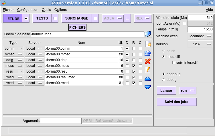
Figure 5.2.3.2-1: Study profile window

5.2.4. Delete a file

To remove a line from the file list, simply select it by clicking in the area where the file name is indicated and clicking on the icon

.

Note:

Only the reference to this file in the astk profile is forgotten, the file itself is not deleted!

5.3. Start the calculation

The data and results files are selected, the calculation parameters are adjusted (see [§ 2.3]), and the « Start » button is clicked.

We take care to check the box just next to ETUDE to indicate that we want to use the content of this tab… otherwise the interface answers « Nothing to launch! »

If the profile has not yet been saved, the interface asks you to choose a location and a name for this profile (see [§ 5.2.3.2]).

astk calls as_run to execute the calculation, and sends the Job Tracker (asjob) the job number (interactive process number) and other information that will allow the progress of the calculation to be monitored. The initial state of the calculation is PEND (pending), when the calculation starts, it becomes RUN, then ENDED when it is finished (other states are possible in batch). The « Refresh » button calls the service that refreshes the status of the current calculations.

When the calculation is complete, you can consult the output of the job by double-clicking on the job, or by*Edit/Output file*.

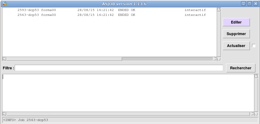
Figure 5.3-1: Job tracking window

5.4. Consultation of the results

You can view the result files simply by double-clicking on their name, which opens a text editor for the « mess » and « resu » files. If you have a result in grace format, « dat », this has the effect of opening this file directly in the grace curve plotter. We thus visualize the curves (displacement as a function of time, stress-deformation…) (provided that grace has been installed, and that « dat » is in the file types associated with*grace*).

NB:

• The directory to host a result file does not exist, it is automatically created if the permissions are sufficient.

• If the copy of the result files fails (problem with permissions, quota, remote connection…), they are copied into a temporary directory on the execution machine. An alarm <A>_ COPY_RESULTS indicates the path where to go to get the results.

5.5. Use of tools

You can also use astk and the fact that you can freely define tools there to gather in a profile all the files necessary for a study even if they are not directly used by*Code_Aster*.

Example: Drawing a curve with grace

We specify the name /home/tutorial/forma00.dat. The file is produced by execution, so we check the « R » box (result) and we uncheck « D » and the logical unit number set to 21. If in the command file we have indicated:

IMPR_COURBE (FORMAT =” XMGRACE “, UNITE =21, COURBE =_F (…)

You can open the curve directly by doing Open with… /grace (right click on the file name), modify the geometry or the mesh parameters.

Of course, this is not limited to grace; you can use other tools (elsewhere, post-processing tools,…) directly from astk and thus access all the files of a study from a profile with the appropriate tool.

5.6. Advanced features

5.6.1. Exectool

In astk, you choose the version of Code_Aster, the debug or nodebug mode, a possible overload and this will lead to the use of this or that Code_Aster executable.

We can go even further by specifying the exact way to launch this executable: this is the role of the exectool launch option (Options menu).

Usually, Code_Aster is started with a command like:

. /aster.exe argument1 argument2…

Using the exectool option is the same as running:

cmde_exec. /aster.exe argument1 argument2…

In the Options menu, you can specify cmde_exec directly or a tool name defined in the as_run configuration file: [ASTER_ROOT] /etc/codeaster/asrun

Example 1:

In the Options menu, enter exectool: time in the box

So the launch command will be time aster.exe arguments…

The time command accepts exactly this type of argument (an executable and its arguments), so we will have the time to execute the calculation. This is not a big step, Code_Aster already gives this type of information.

Example 2:

In the configuration file [ASTER_ROOT] /etc/codeaster/asrun, we define (on a single line):

memcheck: valgrind –tool=memcheck –error-limit=no –leak-check=full –suppressions=/opt/aster/valgrind-python.supp

Then all you have to do is specify exectool: memcheck in the Options menu

memcheck is defined in the configuration file (to the left of the « : »), so the complete valgrind… command will be used during launch.

You can define as many tools as you want as long as you do not conflict with the other parameters defined in this file. For this reason, the definition of « exectools » should evolve in the future.