2. Renumbering and symbolic factorization: MLTPRE#
For convenience, the prefix NU has been omitted in front of the structure names.
Data structures read.
From the data structure: nume_ddl, we extract the records:
NUME. DELG: Indicates whether the degree of freedom is « Lagrange » or not.
NUME. DEEQ,
NUME. NUEQ,
NUME. PRNO: These 3 recordings establish the links between the degrees of freedom subject to a boundary condition and the corresponding Lagranges.
The next 3 records describe a « Morse » matrix.
SMOS. SMHC: Term column number
SMOS. SMDI: Addresses of diagonal terms
SMOS. SMDE.: Numbers of unknowns, and terms in the matrix
Written data structures.
(In front of each Code_Aster structure, we wrote the name of the corresponding table FORTRAN, which will be used later for more convenience.)
MLTF. ADNT ADINIT: addresses of the initial terms in the factored matrix
MLTF. LGBL LGBLOC: length of the blocks of the factored matrix
MLTF. LGSN LGSN: length of the supernodes
MLTF. LOCL LOCAL: used in assembling front matrices, correspondence between the local numbers of the father and son supernode.
MLTF. ADRE ADRESS
MLTF. SUPN SUPND: definition of supernodes
MLTF. FILS FILS: son of the supernodes in the elimination tree
MLTF. FRER FRERE: brother of the supernodes in the elimination tree
MLTF. LGSN LGSN: length of the supernodes
MLTF. LFRN LFRONT: order of the frontal matrices (after elimination)
MLTF. NBAS NBASS: pointer linked to the assembly of the front matrices
MLTF. ADPI ADPILE: addresses in the front-end matrix stack
MLTF. ANCI ANC: inverse renumbering table
MLTF. NBLI NBLIGN: order of the frontal matrices (before elimination)
MLTF. NCBL NCBLOC: number of degrees of freedom for each block
MLTF. DECA DECAL: offset between the start of the column of a supernode and the start of the block JEVEUX that contains it
MLTF. SEQU SEQ: order of elimination of supernodes (tree path).
These data structures will be described in the following paragraphs.
Code description.
There are 2 phases, the first consists in renumbering, the second in what is called in the language of the multi-frontal method, symbolic factorization.
Data structure NUME_DDL describes a numbering of \(\text{NEQ}\) degrees of freedom, including, most of the time, so-called Lagrange degrees of freedom. These degrees of freedom must satisfy the following order relationship:
\(\mathit{L1}<U<\mathit{L2}\), if \(\mathit{L1}\) and \(\mathit{L2}\) are the « Lagranges » associated with the boundary condition on \(U\).
In order to maintain this order, we will subject only the degrees of freedom that are not « Lagranges » to the renumbering algorithm. The « Lagranges » degrees of freedom are therefore removed and the information concerning them is stored in order to reintegrate them into the new numbering, while satisfying (1).
Routines called (a first brief description of the code).
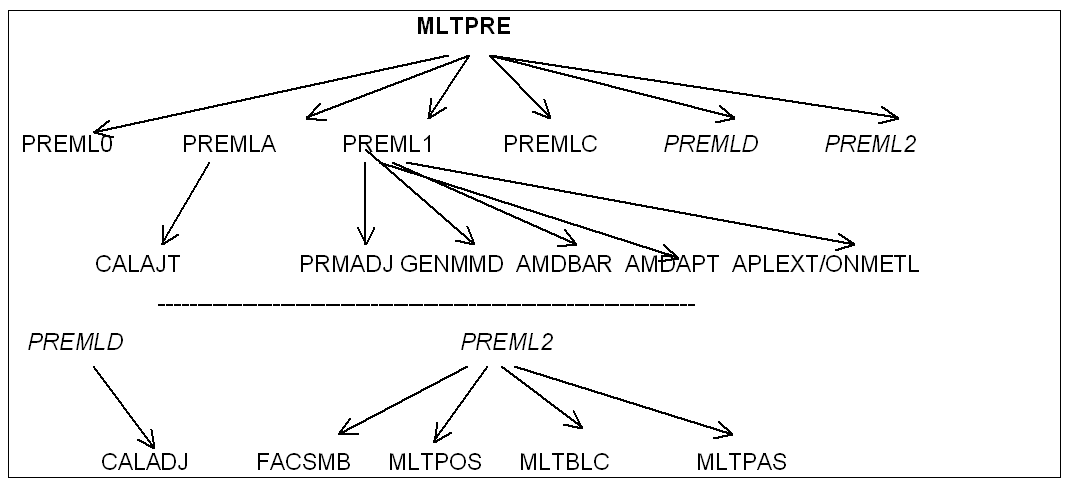
For the first phase, the routines called are as follows:
PREML0: extraction of information on the « Lagranges »
PREMLA: treatment for linear relationship « Lagranges »
PREML1: pre-treatment and renumbering.
PREMLC: post-processing of the renumbering (addition of « Lagranges »).
PREMLD: same
For the second:
PREML2: symbolic factorization.
2.1. PREML0#
The blocking « Lagranges » are stored in tables \(\mathit{LBD1}\), \(\mathit{LBD2}\), and in \(\mathit{RL}\) the linear relationship « Lagranges ».
We get a new numbering from \(1\) to \(\mathit{N2}\) of the degrees of freedom without Lagrange, defined by:
\(P\) of \(\mathrm{[}1\mathrm{:}\text{NEQ}\mathrm{]}\mathrm{\Rightarrow }\mathrm{[}1\mathrm{-}\mathit{N2}\mathrm{]}\), and \(Q\) Inverse of \(P\).
For \(I\) from \(1\) to \(\text{NEQ}\), if \(I\) is a blocked degree of freedom, \(\mathit{LBD1}(I)\), (resp. \(\mathit{LBD2}(I)\)), is the sound number L1 (resp. \(\mathit{L2}\)).
In the case of \(\mathit{NRL}\) linear relationships, we will have:
\(\mathit{RL}(\mathrm{1,}I)\): \(\mathit{L1}\) of the relationship \(I\),
\(\mathit{RL}(\mathrm{2,}I)\): \(\mathit{L2}\) of the \(I\) relationship.
N.B. Programming
In some routines, we’ll use the variable name \(\mathit{N1}\) instead of \(\text{NEQ}\) .
2.2. PREMLA#
For all degrees of freedom \(\mathit{L2}\) of linear relationship, (second « Lagrange »), its lower-numbered neighbors are known by extracting information from the SMOS data structure. SMHC (table COL).
From this information, PREMLAcrée linked lists (tables DEB, VOIS, SUIT) (tables,,) for the degrees of freedom of linear relationship \(\mathit{L2}\).
Let \(J\) be a degree of freedom included in a linear relationship, \(\mathit{j0}\mathrm{=}\mathit{DEB}(j)\) is the address of the first neighbor of \(J\) in table \(\mathit{VOIS}\), \(\mathit{J1}\mathrm{=}\mathit{SUIV}(\mathit{J0})\) is the address of the next neighbor, \(\mathit{J2}\mathrm{=}\mathit{SUIV}(\mathit{J1})\) is the address of the next neighbor, and so on.
This linked list will be used later in PREML1, for the manufacture of \(\mathit{ADJNCY}\).
N.B. Memory Allowance
The linked list consists of 2 local structures, names NOMVOI and NOMSUI , (created by WKVECT and destroyed at the end of MLTPRE ) .
Their length: \(\mathit{LGLIST}\) , is estimated a priori by PREML0 (output parameter \(\text{LT}\) ), if insufficient, PREMLA *provides an error code, and is called again with structures whose length is*2 times larger. *
2.3. PREML1#
PREML1 calls the following routines:
PRMADJ, GENMMD, AMDBAR, ONMETL.
The essential role of PREML1 is to start renumbering. This, carried out at your choice by: METIS (dissection method), GENMMD (minimum degree) or AMDBAR (improved minimum degree), requires 2 prior actions.
2.3.1. Reconstitution of nodes (in the sense of discretization by finite elements).#
In a first version of the code, the renumbering algorithm worked on the \(\mathit{N2}\) degrees of freedom (without Lagranges).
We then wanted to preserve the internal order of the unknowns within the finite element discretization nodes (for example \(\mathit{ux}\), \(\mathit{uy}\), \(\mathit{uz}\), \(p\)).
A development has been carried out for this purpose. On now subjects all the nodes to the renumbering algorithm and not the \(\mathit{N2}\) degrees of liberty.
We therefore form a new set of \(\mathit{NBND}\) nodes and 2 associated pointers:
\(\mathit{NŒUD}\mathrm{[}\mathrm{1 }\mathrm{:}\mathit{N2}\mathrm{]}\mathrm{\Rightarrow }\mathrm{[}\mathrm{1 }\mathrm{:}\mathit{NBND}\mathrm{]}\), and the reverse pointer \(\mathit{DDL}\mathrm{[}\mathrm{1 }\mathrm{:}\mathit{NBND}\mathrm{]}\)
We thus have 3 numberings:
Initial numbering from \(1\) to \(\text{NEQ}\),
That of the degrees of freedom without Lagranges \(1\) to \(\mathit{N2}\),
That of interpolation nodes \(1\) to \(\mathit{NBND}\).
Equipped with tables \(P\) and \(Q\) between the first and the second, \(\mathit{NŒUD}\) and \(\mathit{DDL}\) between the second and the third.
2.3.2. Creating the structure (\(\mathit{ADJNCY}\), \(\mathit{XADJ}\))#
This structure is the standard data structure for the renumbering algorithms mentioned above. We have 2 tables \(\mathit{ADJNCY}\) and \(\mathit{XADJ}\) defined as follows:
Being a \(I\) node, its neighbors are stored in table \(\mathit{ADJNCY}\), between the addresses \(\mathit{XADJ}(I)+1\) and \(\mathit{XADJ}(I+1)\).
First, we create a \((\mathit{ADJNCY},\mathit{XADJ})\) structure relating to the \(\mathit{N2}\) degrees of freedom, then the routine PRMADJ transforms it into a structure \((\mathit{ADJNCY},\mathit{XADJD})\) relating to the \(\mathit{NBND}\) nodes.
To create \(\mathit{ADJNCY}\), we use the \((\mathit{DEB},\mathit{VOIS},\mathit{SUIT})\) linked list created by PREMLA, by forcing the degrees of freedom of a linear relationship to be neighbors. So these degrees of freedom will be in the same super node, as will their \(\mathit{L2}\). The order relationship will thus be respected.
We then make the call to GENMMD, AMDBAR, or METIS. The usual results of this algorithm are obtained:
Renumbering,
Definition of supernodes,
Arborescence
The sources of these 3 methods are in the public domain.
Regarding the last 2 points, they had to be adapted. Renumbering concerns nodes (\(1\) to \(\mathit{NBND}\)), it has the form of 2 tables that are the opposite of each other: \(\mathit{INVPND}\), \(\mathit{PERMND}\). (\(\mathit{INVPND}(I)\) is the new node number \(I\)).
The tree, on the other hand, focuses on the supernodes created by renumbering. Supernode \(\mathit{SND}\) is defined as follows: it consists of node segment \(\mathrm{[}\mathit{SPNDND}(\mathit{SND}\mathrm{-}1)+\mathrm{1,}\mathit{SPNDND}(\mathit{SND})\mathrm{]}\). \(\mathit{SPNDND}\) is thus an injection from segment \(\mathrm{[}\mathrm{1 }\mathrm{:}\mathit{NBSND}\mathrm{]}\) to \(\mathrm{[}\mathrm{1 }\mathrm{:}\mathit{NBND}\mathrm{]}\), \(\mathit{NBSND}\): number of supernodes.
The tree is defined as follows: \(\mathit{PARENT}(\mathit{SND})\) is the « father » node of supernode \(\mathit{SND}\).
N.B. Programming
The multi-front end supernode tree appears under 2 names: \(\mathit{PARENT}\) and \(\mathit{PAREND}\)
The first contains the tree of SNs excluding Lagrange, it is provided by renumbering ( GENMMD/AMDBAR/METIS . )
The second is the complement of the first by adding the Lagranges, it is calculated by PREMLC starting from the first.
In the program calling MLTPRE, \(\mathit{PARENT}\), which is an intermediary, is stored in \(\mathit{ZI}\) at the address \(\mathit{SEQ}\), reused later (saving space).
These previous tables are defined according to the \(\mathit{NBND}\) discretization nodes of*Code_Aster*, (\(1\) to \(\mathit{NBND}\)). They are then rebuilt in the numbering of the \(\mathit{N2}\) degrees of freedom not « Lagrange ».
So \(\mathit{INVPND}\) becomes \(\mathit{INVP}\), \(\mathit{PERMND}\) becomes \(\mathit{PERM}\), and \(\mathit{SPNDND}\) becomes \(\mathit{SUPND}\). (See loops 400 405 406 407 from PREML1).
N.B. Memory Allocation
The structure \((\mathit{XADJ},\mathit{ADJNCY})\) of PREML1 , is called \((\mathit{XADJ2},\mathit{ADJNC2})\) in MLTPRE. It is created before PREML1 and destroyed afterwards. The length of \(\mathit{ADJNC2}\) , \(\mathit{LGADJN}\) , * is estimated to \(2\mathrm{\times }(\mathit{lmat}\mathrm{-}\text{neq}+\mathit{lglist})\) , with \(\mathit{lglist}\) = length of the neighbor list used in PREML0
\(\mathit{lmat}\) = length of the initial matrix (provided by SMOS ) .
If \(\mathit{LGADJN}\) is insufficient, PREML1 provides the required length in return code, and is restarted.
NB. METIS
Previously, we produced a software executable METIS , written in C, compiled and linked separately. This executable was called through APLEXT , the call layer of an external executable by Code_Aster. Now the routines of METIS are compiled and called by a call to ONMETL , calling C function.
2.4. PREMLC#
At the output of PREML1, the results are expressed in terms of non- » Lagrange » degrees of freedom (\(1\) to \(\mathit{N2}\)), the routine PREMLC completes the numbering from \(1\) to \(\mathit{N2}\) by adding the « Lagrange » and by creating new supernodes.
The « Lagranges » are included in the new numbering as follows:
For each \(\mathit{L1}\), a new \(\mathit{SN}\) supernode is created, consisting of a single degree of freedom (\(\mathit{L1}\)), and the son of the first degree of freedom of which it is the « Lagrange » (locked or linear relationship). By being the son of this degree of freedom, he will be eliminated before, which is the rule.
For \(\mathit{L2}\), we don’t create a new \(\mathit{SN}\), we just add an additional degree of freedom (\(\mathit{L2}\)) to the supernode containing the degree of freedom (locked or R.L.) of which it is the « Lagrange ».
In case of a linear relationship, all the degrees of freedom of the relationship are put by the algorithm into the same supernode. This is achieved in the previous paragraph (PREML1), during the fabrication of the \(\mathit{ADJNCY}\) structure, by forcing the degrees of freedom of the linear relationships to be neighboring each other, by means of the linked list (\(\mathit{DEB}\), \(\mathit{VOIS}\), \(\mathit{SUIV}\)).
We get the new renumbers \(\mathit{NOUV}\) and \(\mathit{ANC}\) on \(\mathrm{[}1\mathrm{:}\text{NEQ}\mathrm{]}\), for all degrees of freedom in the new numbering, \(\mathit{ANC}(I)\) will provide its number in the initial numbering. \(\mathit{NOUV}\) is the opposite table.
\(\mathit{NBSN}\) the new number of supernodes and \(\mathit{SUPND}\mathrm{[}1\mathrm{:}\mathit{nbsnd}+1\mathrm{]}\) defines these \(\mathit{SN}\).
Supernode \(\mathit{SN}\) consists of node segment \(\mathrm{[}\mathit{SUPND}(\mathit{SN}\mathrm{-}1)+\mathrm{1,}\mathit{SUPND}(\mathit{SN})\mathrm{]}\).
\(\mathit{SUPND}\) is thus an application from segment \(\mathrm{[}\mathrm{1 }\mathrm{:}\mathit{NBSN}\mathrm{]}\) to \(\mathrm{[}\mathrm{1 }\mathrm{:}\text{NEQ}\mathrm{]}\).
N.B. Memory Allowance
\(\mathit{LGIND}\) is the estimated length of the arrays \(\mathit{GLOBAL}\) AND \(\mathit{LOCAL}\) , (See farther 2.6 ) that are allocated before PREML2 ( \(\mathit{NOPGLO}\) and \(\mathit{NOPLOC}\) )
\(\mathit{LGIND}\) is primarily a result of renumbering, provided by PREML1 and increased by PREMLC depending on boundary conditions.
\(\mathit{LGIND}\) is an overestimation of \(\mathit{GLOBAL}\) and \(\mathit{LOCAL}\) we don’t want to keep a structure that’s too important.
So, after PREML2 , we know the real length of these arrays, we redefine \(\mathit{LGIND}\) to this value, and we copy \(\mathit{GLOBAL}\) and \(\mathit{LOCAL}\) into structures \(\mathit{NOMGLO}\) and \(\mathit{NOMLOC}\) of exact length.
2.5. PREMLD#
This is a technical step: this routine makes a \(\mathit{ADJNCY}\) structure like those used by renumbering algorithms, this time all degrees of freedom from \(1\) to \(\text{NEQ}\) are taken into account.
N.B. Memory Allowance
The structure \((\mathit{XADJ},\mathit{ADJNCY})\) made by PREMLD , is called \((\mathit{XADJ1},\mathit{ADJNC1})\) in MLTPRE.
We use the same length \(\mathit{LGADJN}\) calculated previously.
2.6. PREML2#
This is the second phase of MLTPRE: among other things, we perform symbolic factorization, which is a simulation of real factorization, without floating operation, intended to facilitate the work of real factorization, by manufacturing certain necessary pointers.
PREML2 calls the following routines:
FACSMB: symbolic factorization itself.
MLTPOS: fabrication of the factorization sequence, i.e., raising the tree defined by table \(\mathit{PAREND}\), which thus defines the order in which supernodes are eliminated.
MLTBLC: We define here the division into blocks of the factored matrix, virtually « out of core », because it is divided into blocks that can be released by the JEVEUX software package.
MLTPAS: Here we calculate the address of the initial coefficients in the factored matrix.
2.6.1. FACSMB#
Data (They are the result of renumbering):
\(\mathit{SUPND}\)
\(\mathit{PAREND}\),
(And from the initial topology):
\(\mathit{ADJNCY}\).
Results:
\(\mathit{GLOBAL}\)
\(\mathit{LOCAL}\)
\(\mathit{ADRESS}\)
\(\mathit{NBASS}\)
\(\mathit{DEBFAC}\)
\(\mathit{DEBFSN}\)
\(\mathit{LGSN}\)
\(\mathit{LFRON}\)
\(\mathit{FILS}\)
\(\mathit{FRERE}\).
These tables are described below.
\(\mathit{FILS}\) and \(\mathit{FRERE}\) are the « inverse » arrays of table \(\mathit{PAREND}\), they allow you to know all the « child » supernodes of a given supernode \(\mathit{SN}\), they are \(\mathit{FILS}(\mathit{SN})\), \(\mathit{FRERE}(\mathit{FILS}(\mathit{SN}))\), and so on. For the other results, it is necessary to return to the basic principles of the multi-frontal method, using the following figures:
|
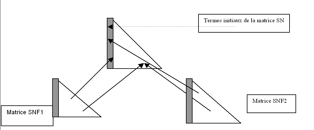
Figure 1 Assembling 2 daughter matrices into a mother matrix
|
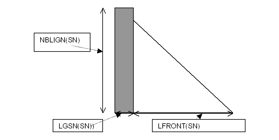
Figure 2 Front matrix \(\mathit{SN}\)
FIG. 1 shows the frontal matrix \(\mathit{SN}\) (of the supernode \(\mathit{SN}\)), consisting of the terms coming from the initial matrix, as well as the terms coming from the daughter matrices \(\mathit{SNF1}\) and SNF2, after eliminating the supernodes \(\mathit{SNF1}\) and \(\mathit{SNF2}\). After elimination, the gray part of the front matrix will constitute the columns of the factored matrix, and the remaining white part stored in the stack of front matrices will agglomerate to the mother matrix during the assembly of this last one.
The symbolic factorization performed by FACSMB will simulate this assembly/elimination process. For each supernode \(\mathit{SN}\), we will create a linked list containing the unknown numbers of the supernode itself, as well as the unknown numbers of the neighbors of all the sons of \(\mathit{SN}\). Neighbors of the sons are included, but not the sons themselves who have been eliminated.
In FORTRAN language, FACSMB produces the following tables:
\(\mathit{LGSN}(\mathit{SN})\): number of unknowns of the supernode \(\mathit{SN}\) (in fact = \(\mathit{supnd}(\mathit{sn}+1)\mathrm{-}\mathit{supnd}(\mathit{sn})\)),
\(\mathit{NBLIGN}(\mathit{SN})\): total number of unknowns of the SN front-end matrix
\(\mathit{LFRONT}(\mathit{SN})\mathrm{=}\mathit{NBLIGN}(\mathit{SN})\mathrm{-}\mathit{LGSN}(\mathit{SN})\), order of the front-end matrix after elimination that will be stored in the stack.
FACSMB also makes an array \(\mathit{GLOBAL}\), equipped with an array of \(\mathit{ADRESS}\) pointers.
\(\mathit{GLOBAL}\) contains the numbers of the unknowns of the front-end matrix \(\mathit{SN}\) (before elimination), between the addresses \(\mathit{ADRESS}(\mathit{SN})\) and \(\mathit{ADRESS}(\mathit{SN}+1)\mathrm{-}1\).
These unknowns are \(\mathit{NBLIGN}(\mathit{SN})\mathrm{=}(\mathit{ADRESS}(\mathit{SN}+1)\mathrm{-}\mathit{ADRESS}(\mathit{SN}))\) in number.
Table \(\mathit{LOCAL}\) is accessed as \(\mathit{GLOBAL}\), using table \(\mathit{ADRESS}\). Let \(\mathit{FSN1}\) be the supernode « son » of the supernode \(\mathit{SN}\), as in the figure above, and let \(I\) be an index between \(\mathit{ADRESS}(\mathit{FSN1})+\mathit{LGSN}(\mathit{FSN1})\) and \(\mathit{ADRESS}(\mathit{FSN1}+1),\mathit{LOCAL}(I)\) will be the local number (between \(1\) and \(\mathit{NBLIGN}(\mathit{SN})\)) of this unknown in the matrix of the supernode « father » \(\mathit{SN}\) (we have \(\mathit{PAREND}(\mathit{FSN1})\mathrm{=}\mathit{SN}\)).
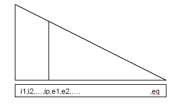
\(\mathit{LOCAL}\) will be used in assembling the « daughter » front-end matrix into the « parent » front-end matrix, it gives the destination address directly. This is illustrated using the following example:
|
Front-end matrix \(\mathit{SN}\) has \((p+q)\) unknowns: \(\mathit{i1},\mathit{i2},\mathrm{..},\mathit{ip},\mathit{e1},\mathit{e2},\dots ,\mathit{eq}\), with
\(\mathit{NBLIGN}(\mathit{SN})\mathrm{=}p+q\)
\(\mathit{LGSN}(\mathit{SN})\mathrm{=}p\)
\(\mathit{LFRONT}(\mathit{SN})\mathrm{=}q\)
\(\mathit{ADRESS}(\mathit{SN}+1)–\mathit{ADRESS}(\mathit{SN})\mathrm{=}p+q\),
\(\mathit{GLOBAL}\mathrm{=}\mathrm{[}\mathit{i1},\mathit{i2},\dots \mathit{ip},\mathit{e1},\mathit{e2},\dots \mathrm{..}\mathit{eq}\mathrm{]}\), with addresses varying between \(\mathit{ADRESS}(\mathit{SN})+1\) and \(\mathit{ADRESS}(\mathit{SN}+1)\),
\(\mathit{LOCAL}\mathrm{=}\mathrm{[}\mathrm{0,0},\mathrm{..},\mathrm{0,}\mathit{l1},\mathit{l2},\dots \dots \mathrm{.}\mathit{lq}\mathrm{]}\)
At the same addresses as above, \(\mathit{l1},\mathit{l2},\mathit{lq}\) are the local numbers in the \(\mathit{PAREND}(\mathit{SN})\) front-end matrix. (values between \(1\) and \(\mathit{NBLIGN}(\mathit{PAREND}(\mathit{SN}))\)).
\(\mathit{NBASS}\), a counter also used for assembly, is defined as follows: \(\mathit{NBASS}(\mathit{FSN1})\) is the number of unknowns \(\mathit{INC}\) such as \(\mathit{INC}<\mathit{SUPND}(\mathit{SN}+1)\), where \(\mathit{PAREND}(\mathit{FSN1})\mathrm{=}\mathit{SN}\). So this is the number of unknowns in \(\mathit{FSN1}\), assembled in the mother matrix \(\mathit{SN}\) and which will be eliminated when \(\mathit{SN}\) is eliminated.
\(\mathit{DEBFAC}\) and \(\mathit{DEBFSN}\), these 2 tables give the same values, the first is indexed by unknown, the second by supernode, they provide, for \(\mathit{DEBFAC}\), the addresses of the diagonal coefficients of the unknowns in the factored matrix. For \(\mathit{DEBFSN}\), this is the address of the diagonal coefficient of the first unknown of the supernode.
We saw in Figure 2 that the columns corresponding to the unknowns of the eliminated supernode, (in gray), constituted the columns of the factored matrix called \(\mathit{FACTOR}\). The addresses of the diagonal coefficients provided by DEBFAC are addresses in a virtual array \(\mathit{FACTOR}\) containing the factored matrix. In fact, a set of JEVEUX blocks will contain the factored matrix, and an additional pointer will be used for each block.
N.B. Programming
We can see in the previous figures that we store the columns of \(\mathit{SN}\), all integer, (gray rectangle), without taking into account the symmetry of the diagonal block. We thus consume a little more memory, but we are dealing with regular storage necessary for the use of routines BLAS which require storages in 2-dimensional FORTRAN arrays.
2.6.2. MLTPOS#
It should be noted that the frontal matrices resulting from the removals are stored in a stack. All the daughter matrices of the same super node \(\mathit{SN}\) are stored (stacked), consecutively. Once read (unstacked), they are no longer reused, and the front-end matrix resulting from the elimination of \(\mathit{SN}\) is stored in their place. The length of this pile decreases or increases as you kill it, it reaches a maximum that you need to know.
MLTPOS goes through the tree, calculates \(\mathit{ESTIM}\), the maximum length of the stack for its subsequent allocation, constructs an array \(\mathit{SEQ}(\mathrm{1 }\mathrm{:}\mathit{NBSN})\) that provides the order of elimination of supernodes by going through the tree from the bottom up. It provides \(\mathit{ADPILE}\) which contains the address in the stack of the \(\mathit{SN}\) front-end matrices.
MLTPOS contains an algorithm for renumbering the order in which supernodes are eliminated, intended to minimize the length of the front-end matrix stack ([AS87])
2.6.3. MLTBLC#
This routine builds the pointers for the block division of the factored matrix. Each block will contain the columns of an integer number of supernodes. We will never encounter the configuration where the different columns of the same supernode belong to 2 blocks.
Data:
\(\mathit{MAXBLOC}\): maximum block length. Each block will contain columns for as many super nodes as possible. \(\mathit{MAXBLOC}\) is calculated before the call to MLTBLC, it is in fact the length (in columns) of the largest of the supernodes, and the latter (generally the highest in the tree) will occupy a block by itself.
Results:
\(\mathit{NBLOC}\): Number of blocks.
\(\mathit{LGBLOC}(\mathrm{1 }\mathrm{:}\mathit{NBLOC})\): lengths of each block.
\(\mathit{NCBLOC}(\mathrm{1 }\mathrm{:}\mathit{NBLOC})\): definition of the blocks, as follows block \(\mathit{IB}\) consists of the columns of the supernodes \(\mathit{SEQ}(\mathit{NCBLOC}(\mathit{IB}\mathrm{-}1)+1)\), to \(\mathit{SEQ}(\mathit{NCBLOC}(\mathit{IB}))\).
\(\mathit{DECAL}(\mathrm{1 }\mathrm{:}\mathit{NBSN})\) lag table that allows access to the first diagonal term of each supernode in the factored matrix. We will illustrate this with the following diagram:
ISN =0
For IB=1, NBLOC! Loop over the blocks of the factored
JEVEUO (JEXNUM (FACTOL, IB), “L”, IFACL)
! Block IB from collection FACTOL is loaded in IFACL
For NC = 1, NCBLOC (IB)! Loop on the Supernodes of Block IB
ISN = ISN +1
SN= SEQ (ISN)! We follow the elimination sequence
ADFAC = IFACL + DECAL (SN) —1
! ADFAC is the address in ZR of the first coefficient of the supernode SN
2.6.4. MLTPAS#
This routine calculates the addresses in the factored matrix, coefficients from the initial matrix.
These addresses are stored in structure MLTF. ADNT, whose name is FORTRAN \(\mathit{ADINIT}\) or \(\mathit{COL}\) and whose length is \(\mathit{LMAT}\).
N.B. Programming particularity.
Some addresses calculated of \(\mathit{ADINIT}\) are negative. Indeed in the non-symmetric case, we have 2 initial matrices \(\mathit{MATI}\) and \(\mathit{MATS}\) which have the same topology, (same neighbors, same trough), the symbolic factorization is the same.
However, it may happen that a coefficient of \(\mathit{MATI}\) (lower part of the initial matrix), has a destination in the upper part of the factored matrix. (In the same way between \(\mathit{MATS}\) and the lower part of the factorized one). In this case the address of the initial coefficient is stored negative and the routine for injecting the coefficients of the initial matrix, * MLTASAle takes into account and addresses the coefficients correctly.
IF (CODE .GT.0) THEN
ZR (IFACL + ADPROV - DEB) = ZR (MATI +I1-1): MATI injected into IFACL (ower)
ZR (IFACU + ADPROV - DEB) = ZR (MATS +I1-1)
ELSE
ZR (IFACL + ADPROV - DEB) = ZR (MATS +I1-1)
ZR (IFACU + ADPROV - DEB) = ZR (MATI +I1-1) MATI injected into IFACU (pper)
ENDIF
2.7. MLTPRE call tree#
|