3. Numerical factorization MULFR8#
We are dealing with factorization itself, the routines called are:
MLTPRE
MLTASA
MLTFC1
MLTPRE, seen earlier, is called if needed. We check that it has not already been called beforehand, in this case we go out of the routine.
3.1. MLTASA#
This routine injects the initial terms of the matrix into the factored matrix. Table \(\mathit{ADINIT}\) calculated previously by MLTPRE provides the addresses.
Data:
The recording. VALM of the NOMMAT sd_matr_asse structure provided.
\(\mathit{ADINIT}\) and \(\mathit{LGBLOC}(\mathrm{1 }\mathrm{:}\mathit{NBLOC})\) calculated by MLTPRE.
Results:
MLTASA creates a scattered collection with the name \(\mathit{FACTOL}\) having \(\mathit{NBLOC}\) blocks of lengths given by \(\mathit{LGBLOC}(\mathrm{1 }\mathrm{:}\mathit{NBLOC})\).
In the non-symmetric case, the routine reads 2 ». VALM » with respective names \(\mathit{MATI}\) and \(\mathit{MATS}\), lower and upper parts of the initial matrix, and creates 2 collections \(\mathit{FACTOL}(\mathit{ower})\) and \(\mathit{FACTOU}(\mathit{pper})\).
3.2. MLTFC1#
We are in the case where the stack of front matrices is stored in an array FORTRAN named \(\mathit{PILE}\) and allocated by WKVECT in the caller MULFR8, this array is destroyed at the end of the routine.
A version with the front matrices in a scattered collection has been written (MLTFCB), but is not used.
MLTFC1 has the following structure:
In an external loop on the blocks of the factored,
Loading the block into memory
Loop on the nodes of the block
\(\mathit{SEQ}\) provides the order of elimination
Supernode \(\mathit{SNI}\) is therefore eliminated in various phases:
Assembling « daughter » matrices using MLTAFF and MLTAFF
Elimination of the columns of \(\mathit{SNI}\) that are the columns of the factorized: MLTFLM
Update the remaining unknowns in the front-end matrix (Schur complement): MLTFMJ
End of loop
End of loop
For IB=1, NBLOC! Loop over the blocks of the factored
JEVEUO (JEXNUM (FACTOL, IB), “L”, IFACL)
! Block IB from collection FACTOL is loaded in IFACL
For NC = 1, NCBLOC (IB)! Loop on the Supernodes of Block IB
ISN = ISN +1
SNI = SEQ (ISN)
For all the SN sons of SNI! Assembling daughter matrices
mltafp
Mtaff
! End of the assembly of the daughter matrices
mltflm! elimination of the SN: factorization on the columns of the SN
mltfmj! Contribution of the columns eliminated on the other degrees of freedom of the front, update of the frontal matrix
! End of loop on super knots
! End of loop on the blocks
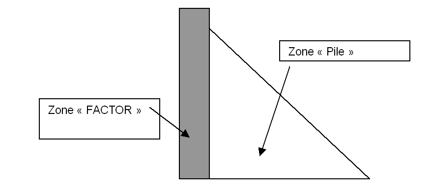
Before describing the routines called, it is necessary to specify how the matrix is arranged. We look at the following diagram:
|
Figure 3 Breakdown of the front matrix into 2 storage areas
The gray rectangular part represents the « active area of the front matrix », it is the columns of \(\mathit{SN}\) that will be eliminated, and will constitute the columns of the factorized matrix \(\mathit{FACTOR}\). To avoid a memory copy between the front matrix and \(\mathit{FACTOR}\), we store the coefficients directly in \(\mathit{FACTOR}\), we will say that it is the « \(\mathit{FACTOR}\) » part of the front matrix. Besides, we have the « passive » zone of the front matrix, (Schur complement in fact), which will be stored in the stack, in the same way, to avoid a memory copy, this part of the matrix is stored directly in the stack.
Mltafrp and mltaff are the routines that assemble the « daughter » front-end matrices into the « parent » front-end matrix.
3.2.1. MLTAFP#
This routine assembles the coefficients of the « daughter » frontal matrix, in the « \(\mathit{FACTOR}\) » zone of the « mother » frontal matrix.
3.2.2. Mltaff#
This routine copies the coefficients of the « daughter » front-end matrix into the « stack » zone of the « parent » front-end matrix.
3.2.3. MLTFLM#
Elimination of super node \(\mathit{SN}\), i.e. partial factorization of the front matrix, work in zone « \(\mathit{FACTOR}\) ».
mltflm calls:
dgemv: Blas routine that performs matrix*vector products
mltfld (call to DGEMV)
mltflj (call to DGEMM).
3.2.4. MLTFMJ#
Update to the « \(\mathit{PILE}\) » zone which is modified by the elimination of \(\mathit{SN}\).
mltfmj calls:
dgemm: Blas routine that produces matrix-matrix products.
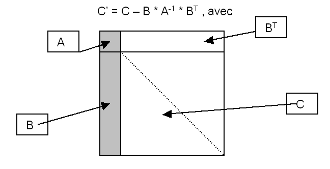
mltfmj is the routine that consumes the most calculation time, it updates the frontal matrix on the rows and columns of the degrees of freedom similar to those eliminated, it is an operation that can be written:
|
In order to reduce the calculation costs, the matrices \(A\), \(B\) and \(C\) are virtually divided into sub-blocks of order \(\mathit{NB}\) and the operation (1) above is performed in blocks by calling the Blas DGEMM routine. This routine optimized by the manufacturer on each machine takes advantage of the fact that the small blocks of order \(\mathit{NB}\) multiplied in this way fit in the primary cache, thus reducing memory access costs. \(\mathit{NB}\) is currently set to 96, this value generally of the order of a few dozen depends on the size of the \(\mathit{L1}\) cache, the closest to the processor, and on the size of the problems treated. It could be re-estimated from time to time according to new machine acquisitions, on a set of significant test cases. The tests carried out previously showed that the performances varied little when NB varied around 96.
mltflm also uses this block division and uses DGEMM through mltflj. (In the case where the number of columns to be eliminated is less than a certain threshold (\(\mathit{pmin}\mathrm{=}10\)), the call to these last 2 routines is replaced by the call to MLFT21). This was done in order to optimize the elimination of « small » supernodes; it would be appropriate to verify that this is still justified. Thus, for the sake of simplification, after verifying the absence of performance degradation for small cases, one could remove this threshold and thus eliminate a subprogram call branch.
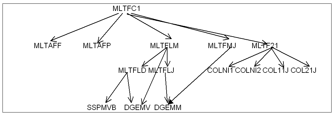
To illustrate this, the tree of routines called in the symmetric case is as follows:
|
Figure 4 Factorization **** (symmetric real case) . **