2. Benchmark solutions#
2.1. Calculation method used for reference solutions#
2.1.1. Modeling A#
The equations governing behavior are nonlinear differential equations. To validate the answer obtained with Code_Aster in non-linear statics, an integration by a Runge-Kutta method is carried out with a tool external to Code_Aster.
The comparison is carried out on the displacement and on the effort, for the 4 types of discrete elements.
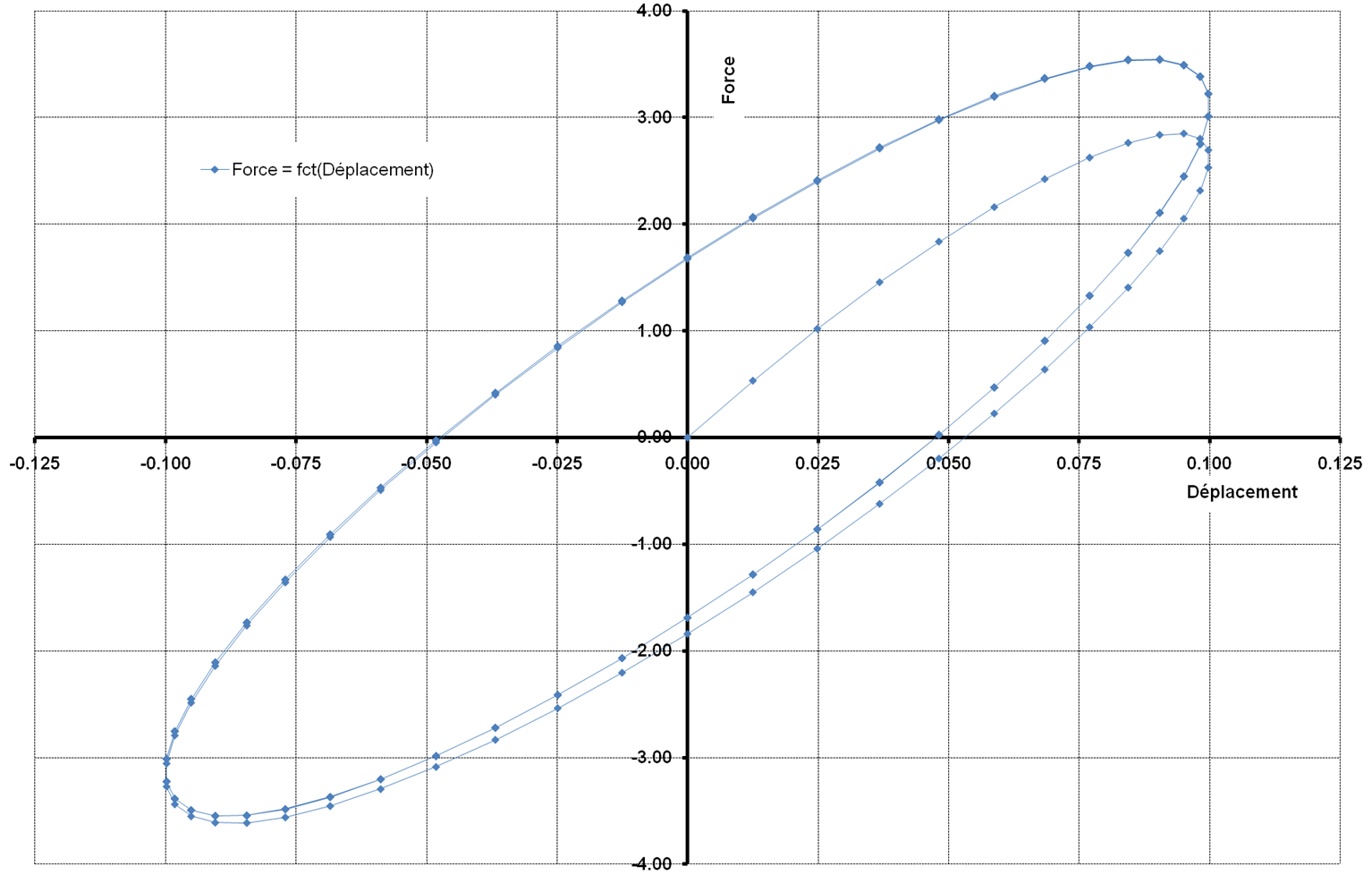
Figure 2.1.1-a : Force displacement curve, modeling A.
The answer given by*Code_Aster* is tested for the following values:
Moment |
Movement \({U}_{x}\) |
Force \({F}_{x}\) |
2.00E-02 |
5.877852523E-02 |
2.187710580E+00 |
4.00E-02 |
9.510565163E-02 |
2.829192223E+00 |
6.00E-02 |
9.510565163E-02 |
2.035749590E+00 |
8.00E-02 |
5.877852523E-02 |
2.402408962E-01 |
1.00E-01 |
-1.653950414E-16 |
-1.851221553E+00 |
1.32E-01 |
-8.443279255E-02 |
-3.445042947E+00 |
2.00E-01 |
4.196133458E-16 |
1.745702939E+00 |
2.32E-01 |
8.443279255E-02 |
3.409095131E+00 |
2.68E-01 |
8.443279255E-02 |
1.626471785E+00 |
3.16E-01 |
-4.817536741E-02 |
-2.962435650E+00 |
3.56E-01 |
-9.8228725072507E-02 |
-2.590008311E+00 |
4.12E-01 |
3.681245527E-02 |
2.724835444E+00 |
4.36E-01 |
9.048270525E-02 |
3.394150679E+00 |
5.20E-01 |
-5.877852523E-02 |
-3.151025904E+00 |
6.24E-01 |
6.845471059E-02 |
3.289283317E+00 |
7.16E-01 |
-4.817536741E-02 |
-2.962278876E+00 |
8.00E-01 |
1.678385621E-15 |
1.750844985E+00 |
8.16E-01 |
4.817536741E-02 |
2.962278875E+00 |
8.48E-01 |
9.980267284E-02 |
3.047135026E+00 |
9.40E-01 |
-9.510565163E-02 |
-3.326860603E+00 |
9.68E-01 |
-8.443279255E-02 |
-1.627037269E+00 |
1.00E+00 |
-1.224606354E-16 |
1.750844985E+00 |
Table 2.1.1-a : Displacement and Forces, modeling A.
2.1.2. B modeling#
This non-linear static modeling makes it possible to test, in addition to the law of behavior, the dissipation during a stabilized cyclic loading. The dissipation is compared to a theoretical value obtained in the particular case \({\alpha }_{3}=1.0\).
Note: For a cyclic loading with \({\alpha }_{3}\ne 1\) the theoretical calculation of the dissipation is not available, except for a stabilized cycle.
The answer given by*Code_Aster* is tested for the following values:
Moment |
Movement \({U}_{x}\) |
Force \({F}_{x}\) |
2.00E-02 |
5.877852523E-02 |
2.160195640E+00 |
4.00E-02 |
9.510565163E-02 |
2.849834733E+00 |
6.00E-02 |
9.510565163E-02 |
2.052734480E+00 |
8.00E-02 |
5.877852523E-02 |
2.258915314E-01 |
1.00E-01 |
-1.653950414E-16 |
-1.838798378E+00 |
1.32E-01 |
-8.443279255E-02 |
-3.611426479E+00 |
2.00E-01 |
4.195726882E-16 |
1.674446965E+00 |
2.32E-01 |
8.443279255E-02 |
3.535539017E+00 |
2.68E-01 |
8.443279255E-02 |
1.730277335E+00 |
3.16E-01 |
-4.817536741E-02 |
-2.984761046E+00 |
3.56E-01 |
-9.8228725072507E-02 |
-2.752278435E+00 |
4.12E-01 |
3.681245527E-02 |
2.719185079E+00 |
4.36E-01 |
9.048270525E-02 |
3.544941424E+00 |
5.20E-01 |
-5.87785252523E-02 |
-3.201565830E+00 |
6.24E-01 |
6.845471059E-02 |
3.368686714E+00 |
7.16E-01 |
-4.817536741E-02 |
-2.983942123E+00 |
8.00E-01 |
1.678385621E-15 |
1.687931415E+00 |
8.16E-01 |
4.817536741E-02 |
2.983942066E+00 |
8.48E-01 |
9.980267284E-02 |
3.223403140E+00 |
9.40E-01 |
-9.510565163E-02 |
-3.492301297E+00 |
9.68E-01 |
-8.443279255E-02 |
-1.732887550E+00 |
1.00E+00 |
-1.224606354E-16 |
1.687931421E+00 |
Table 2.1.2-a: Displacement and Forces, modeling B.
The calculation of the dissipation over a stabilized cycle is obtained by integrating the equations of the system in the particular case where \({\alpha }_{3}=1\).
On a stabilized cycle, for \({\alpha }_{3}=1\), the dissipation value is:
\(\Delta D=\frac{\pi \mathrm{.}{U}_{0}^{2}\mathrm{.}{E}_{1}^{2}\mathrm{.}{E}_{3}^{2}\mathrm{.}\omega \mathrm{.}{C}_{3}}{{\omega }^{2}\mathrm{.}{C}_{3}^{2}\mathrm{.}{({E}_{1}+{E}_{2}+{E}_{3})}^{2}+{({E}_{1}+{E}_{2})}^{2}\mathrm{.}{E}_{3}^{2}}\) [éq2.1.2-1]
2.1.3. C modeling#
This static nonlinear modeling makes it possible to test the law of behavior during a creep test. Displacement is imposed and remains constant: \({U}_{0}=0.1\). The response of the law of behavior as well as the dissipation are compared to the theoretical values obtained in the particular case \({\alpha }_{3}=0.5\).
The integrated differential equations in the particular case of constant \(U\) and \({\alpha }_{3}=0.5\) give the equations of effort and dissipation as a function of time:
\(F(t)=\frac{{U}_{0}\mathrm{.}{E}_{1}\mathrm{.}({\mathrm{AA}}_{s}+{\mathrm{BB}}_{s}\mathrm{.}{E}_{2}\mathrm{.}t)}{{({E}_{3}+{E}_{2}+{E}_{1})}^{2}\mathrm{.}{C}_{3}^{2}+{\mathrm{BB}}_{s}\mathrm{.}({E}_{2}+{E}_{1})\mathrm{.}t}\) [éq2.1.3-1]
\(D(t)=\frac{{U}_{0}^{3}.{E}_{1}^{3}.{E}_{3}^{3}}{2.({E}_{3}+{E}_{2}+{E}_{1})}.\mathit{t.}\frac{(2.{\mathit{AA}}_{e}+{\mathit{BB}}_{e}.t)}{{({\mathit{AA}}_{e}+{\mathit{BB}}_{e}.t)}^{2}}\) [éq2.1.3-2]
with \(\{\begin{array}{}{\mathrm{AA}}_{s}=({E}_{3}+{E}_{2})\mathrm{.}({E}_{1}+{E}_{2}+{E}_{3})\mathrm{.}{C}_{3}^{2}\\ {\mathrm{BB}}_{s}={U}_{0}\mathrm{.}{E}_{1}\mathrm{.}{E}_{3}^{2}\end{array}\{\begin{array}{}{\mathrm{AA}}_{e}={({E}_{3}+{E}_{2}+{E}_{1})}^{2}\mathrm{.}{C}_{3}^{2}\\ {\mathrm{BB}}_{e}={U}_{0}\mathrm{.}{E}_{1}\mathrm{.}{E}_{3}^{2}\mathrm{.}({E}_{2}+{E}_{1})\end{array}\)
2.1.4. D modeling#
The equations governing behavior are nonlinear differential equations. To validate the answer obtained with Code_Aster in non-linear statics, an integration by a Runge-Kutta method is carried out with a tool external to Code_Aster.
The comparison is carried out on the displacement and on the effort.
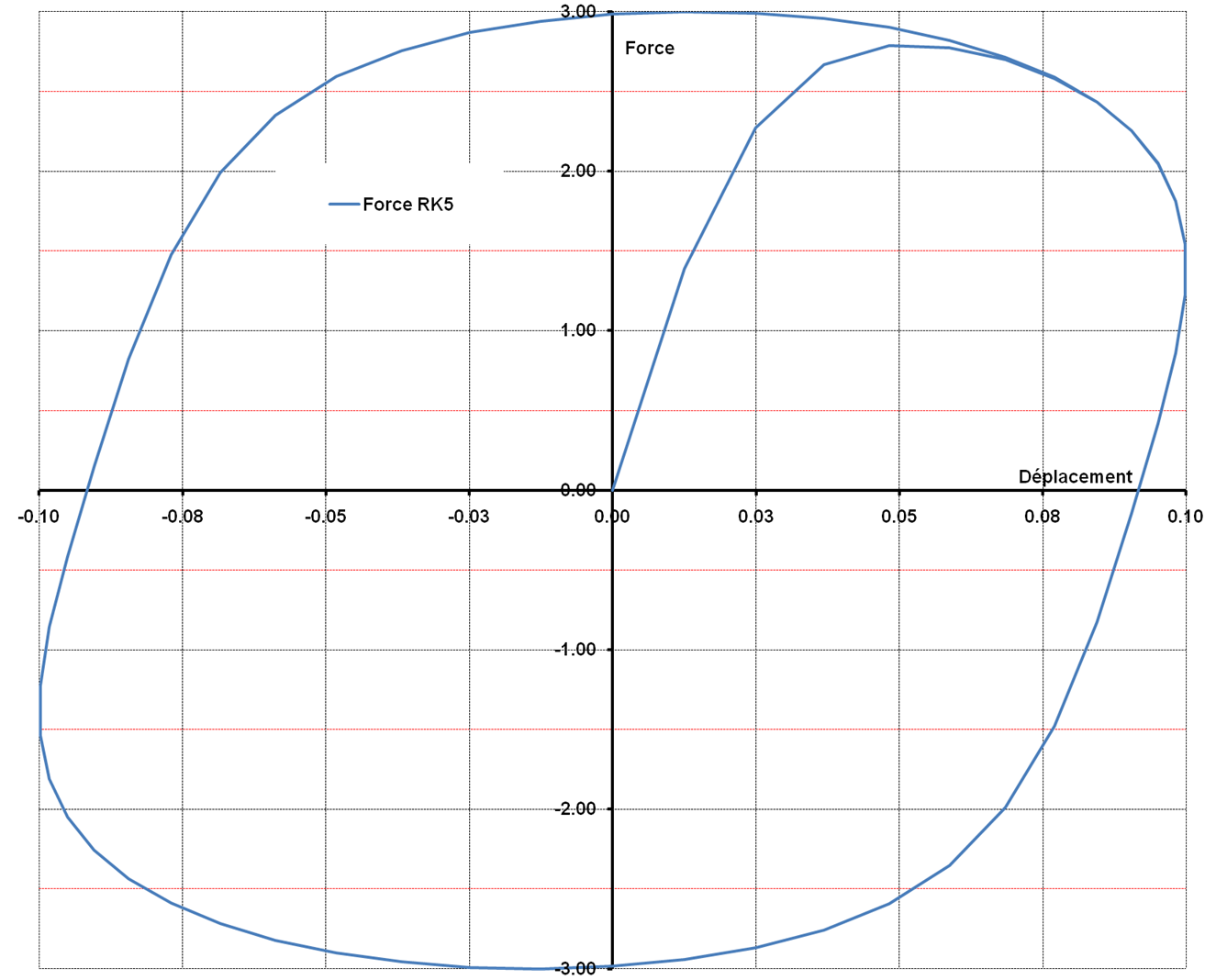
Figure 2.1.4-a : Force displacement curve, modeling D.
The answer given by*Code_Aster* is tested for the following values:
Moment |
Movement \({U}_{x}\) |
Force \({F}_{x}\) |
4.000E-03 |
1.2533323356430E-02 |
1.3901305564654E+00 |
4.800E-02 |
9.9802672872842827E-02 |
1.5399690347096E+00 |
1.000E-01 |
-1.6539504141266E-16 |
-2.9840799981192E+00 |
1.360E-01 |
-9.048270505246602E-02 |
-2.2555706075403E+00 |
2.040E-01 |
1.2533323356431E-02 |
2.9999350282465E+00 |
2.480E-01 |
9.9802672872842827E-02 |
1.5401915597398E+00 |
3.040E-01 |
-1.25333233532356431E-02 |
-2.9999350282852E+00 |
3.480E-01 |
-9.9802672872842827E-02 |
-1.5401915597074E+00 |
4.040E-01 |
1.2533323356431E-02 |
2.9999350282970E+00 |
5.000E-01 |
-1.0045133128078E-15 |
-2.9840798812719E+00 |
5.600E-01 |
-9.5105651629515E-02 |
-4.1551773591104E-01 |
6.000E-01 |
1.3475548801822E-15 |
2.9840798812750E+00 |
6.400E-01 |
9.510565162951629516E-02 |
2.0490126532863E+00 |
7.040E-01 |
-1.25333233523356432E-02 |
-2.9999350283063E+00 |
7.480E-01 |
-9.9802672872842827E-02 |
-1.5401915596821E+00 |
8.040E-01 |
1.2533323356432E-02 |
2.9999350283073E+00 |
8.480E-01 |
9.9802672872842827E-02 |
1.5401915596806E+00 |
9.040E-01 |
-1.253332335323356432E-02 |
-2.9999350283079E+00 |
9.480E-01 |
-9.9802672872842827E-02 |
-1.5401915596795E+00 |
1.000E+00 |
-1.2240642527361E-16 |
2.9840798812793E+00 |
Table 2.1.4-a: Displacement and Forces, modeling D.
2.2. Uncertainty about the solution#
2.2.1. Modeling A#
For the effort response, displacement:
The reference solution is obtained by numerical integration of a nonlinear differential system.
2.2.2. B modeling#
For the effort response, displacement:
The reference solution is obtained by numerical integration of a differential system, with a 5th order Runge-Kutta method.
For dissipation:
No uncertainty, the solution is analytical.
2.2.3. C modeling#
For the effort response, displacement:
No uncertainty, the solution is analytical.
For dissipation:
No uncertainty, the solution is analytical.
2.2.4. D modeling#
For the effort response, displacement:
The reference solution is obtained by numerical integration of a differential system.