1. Reference problem#
1.1. Device description#
The viscous damper is represented by the rheological model below.
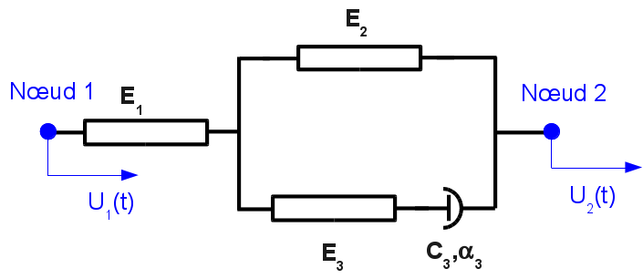
Figure 1.1-a: Rheological model of the viscous damper.
The values of the various stiffness \({E}_{1}\), \({E}_{2}\), \({E}_{3}\) and the characteristics of the non-linear viscous part \({C}_{3}\), \({\alpha }_{3}\) are derived from tests. The equations governing behavior are [R5.03.17]:
\({\dot{F}}_{1}\left(\frac{1}{{E}_{1}}+\frac{1}{{E}_{3}}+\frac{{E}_{2}}{\left({E}_{1}.{E}_{3}\right)}\right)=\left({\dot{U}}_{2}-{\dot{U}}_{1}\right)\left(1+\frac{{E}_{2}}{{E}_{3}}\right)-{\langle \langle \frac{{F}_{1}}{{C}_{3}}\left(1+\frac{{E}_{2}}{{E}_{1}}\right)-\frac{{E}_{2}}{{C}_{3}}\left({U}_{2}-{U}_{1}\right)\rangle \rangle }^{1/{\alpha }_{3}}\)
with \(\begin{array}{cc}{\langle \langle x\rangle \rangle }^{a}={x}^{a}& \mathit{si}x\ge 0\\ {\langle \langle x\rangle \rangle }^{a}=-{∣x∣}^{a}& \mathit{si}x\le 0\end{array}\)
The dissipation increment is:
\(\Delta D={C}_{3}.{∣\frac{{F}_{1}}{{C}_{3}}\left(1+\frac{{E}_{2}}{{E}_{1}}\right)-\frac{{E}_{2}}{{C}_{3}}\left({U}_{2}-{U}_{1}\right)∣}^{1+1/{\alpha }_{3}}\)
1.2. Modelizations#
The models tested are on elements DIS_T then DIS_TR, cells SEG2 then cells POI1. The stiffness characteristics of the discrete elements, which are used for the prediction of the non-linear algorithm, are therefore of the type: K_T_D_L, K_ TR_D_L, K_T_D_N, K_ TR_D_N, K_, depending on the type of element.
Note: The units of the parameters should agree with the unit of effort, the unit of length, and the unit of time of the problem [R5.03.17]. For all models the units are homogeneous to [N], [m], [s].
1.2.1. Modeling A#
This modeling makes it possible to test the non-linear static cyclic behavior of the law.
1.2.2. B modeling#
This modeling in nonlinear statics makes it possible to test, in addition to the law of behavior, the dissipation during a stabilized cyclic loading. The dissipation is compared to a theoretical value obtained in the particular case \({\alpha }_{3}=1.0\). For a cyclic loading with \({\alpha }_{3}\ne 1\) the theoretical calculation of the dissipation is not available.
1.2.3. C modeling#
This static nonlinear modeling makes it possible to test the law of behavior during a creep test. Displacement is imposed and remains constant. The response of the law of behavior as well as the dissipation are compared to the theoretical values obtained in the particular case \({\alpha }_{3}=0.5\).
1.2.4. D modeling#
This modeling validates the fact that it is possible to model a Maxwell shock absorber by affecting the appropriate material characteristics. It is possible to make the stiffness extend to infinity by using the key words UNSUR_K when defining the material. In this specific case \(\mathit{K1}=120.0\), \(\mathit{K2}=0\), \(\mathit{K3}\to \infty\) or \(\mathit{UNSUR}\text{\_}\mathit{K3}=0\). The modelled shock absorber is shown in the following figure.
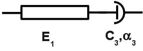
Figure 1.2.4-a: Maxwell shock absorber.
Note: To model this damper, you can also choose the following values \(\mathit{K2}=0\), \(\mathit{K3}=120.0\), \(\mathit{K1}\to \infty\), i.e. \(\mathit{UNSUR}\text{\_}\mathit{K1}=0.0\).
1.3. Material properties#
1.3.1. Modeling A#
\(\mathit{K1}=120.0\), \(\mathit{K2}=10.0\), \(\mathit{K3}=60.0\), \(C=1.7\), \(\mathit{PUIS}\text{\_}\mathit{ALPHA}=0.8\)
1.3.2. B modeling#
\(\mathit{K1}=120.0\), \(\mathit{K2}=10.0\), \(\mathit{K3}=60.0\), \(C=1.7\), \(\mathit{PUIS}\text{\_}\mathit{ALPHA}=1.0\)
1.3.3. C modeling#
\(\mathit{K1}=120.0\), \(\mathit{K2}=10.0\), \(\mathit{K3}=60.0\), \(C=1.7\), \(\mathit{PUIS}\text{\_}\mathit{ALPHA}=0.5\)
1.3.4. D modeling#
\(\mathit{K1}=120.0\), \(\mathit{K2}=0.0\), \(\mathit{UNSUR}\text{\_}\mathit{K3}=0.0\), \(C=1.7\), \(\mathit{PUIS}\text{\_}\mathit{ALPHA}=0.50\)
1.4. Boundary conditions and loads#
When the discrete is a SEG2, one of the nodes is blocked, on the other a displacement condition is imposed. When the discrete is a POI1 the displacement condition is imposed on this node.
The on-the-go condition is a function of time for models A, B, and D:
\({U}_{0}.\mathrm{sin}(2\pi .\mathit{f.t})\) with \(f=5\mathit{Hz}\)
In C modeling, the displacement is imposed and remains constant: \({U}_{0}=0.1\)