2. Reference solution#
2.1. Calculation method#
The reference solution is obtained by integrating the equations of the model in Mathematica for axisymmetric modeling. To do this, it suffices to write the formal equations of the system, to apply to them the transformation rule characterizing Hooke’s law and to solve the nonlinear differential system. Users wishing to obtain more information can refer to the note HT-2C/97/016/A
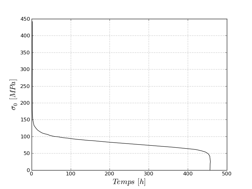
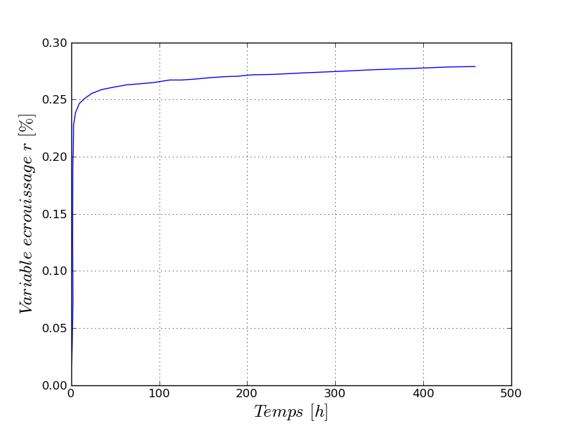
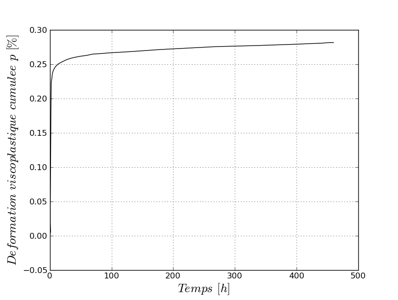
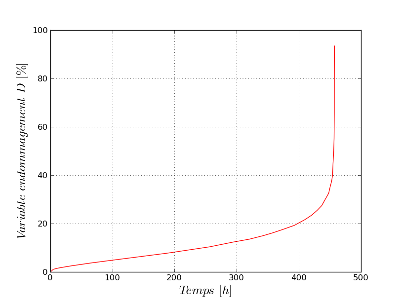
Here are the results of integrating the behavior, depending on the case where the coefficient \({K}_{D}\) is chosen depending on the temperature and on \({\sigma }_{0}\) (modeling a and b):
|
|
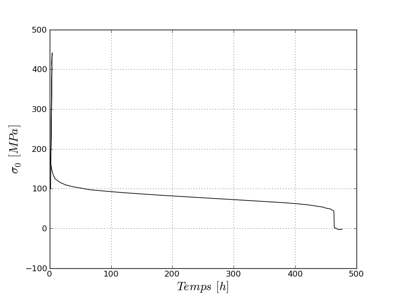
SIGM for K_D (T, SIG) |
r for K_D (T, SIG) |
|
|
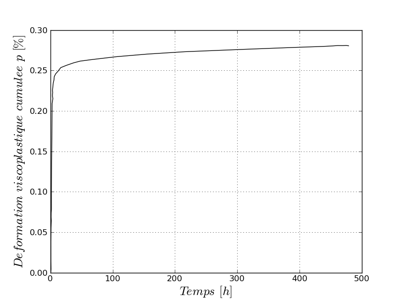
p for K_D (T, SIG) |
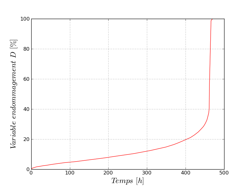
D for K_D (T, SIG) |
Here are the results of integrating the behavior, depending on the case where the coefficient \({K}_{D}\) is chosen depending only on the temperature (c and d modeling):
|
|
SIGM for K_D (T) |
r for K_D (T) |
|
|
p for K_D (T) |
D for K_D (T) |
In the graphs above, \(D\) is the damage variable corresponding to the internal variable \(\mathit{V9}\), \(r\) is the multiplicative viscoplastic work hardening variable corresponding to the internal variable \(\mathit{V8}\), and \(p\) is the cumulative viscoplastic deformation corresponding to the internal variable \(\mathit{V7}\).
We also have the following correspondence, in relation to the parameters of the VENDOCHAB keyword:
\(N\mathrm{=}{N}_{\mathit{VP}}\)
\(M\mathrm{=}{M}_{\mathit{VP}}\)
\(K\mathrm{=}{K}_{\mathit{VP}}\)
\(A\mathrm{=}{A}_{D}\)
\(R\mathrm{=}{R}_{D}\)
\(k\mathrm{=}{K}_{D}\)
2.2. Benchmark results#
The coefficient \({K}_{D}\) is chosen depending on the temperature and on \({\sigma }_{0}\). ~~~~~~~~~~~~~~~~~~~~~~~~~~~~~~~~~~~~~~~~~~~~~~~~~~~~~~~~~~~~~~~~~~~~~~~~~~~~~~~~~~~~~~~~~~~~~~~~~~~~~~~~~~~~~~~~~~~~~~~~~~~~~~~~~~~~~~~~~~~~~~~~~~~~~~~~~~~~~~~~~~~~~~~~~~~~~~~~~~~~~~~~~~~~~~~ ~~
Evolution of the constraint, \({\sigma }_{0}\), as a function of time. This value is tested at various times:
Instant |
Reference |
20 |
252.76091 |
2000 |
164.261 |
200000 |
101.596 |
1000000 |
75.978499999999997 |
1600000 |
55.54209999999999998 |
Table 2.2.1-1 : Benchmark results for K_D (T, SIG)
Evolution of the damage variable, \(D\) as a function of time. This value is tested at various times depending on the modeling:
Instant |
Reference |
20 |
2.3168400000000001E-4 |
2000 |
2.77144E-3 |
200000 |
0.032255100000000002 |
1000000 |
0.110134 |
1600000 |
0.28131600000000001 |
Table 2.2.1-2 : Benchmark results for K_D (T, SIG)
Evolution of the viscoplastic isotropic work hardening variable, \(r\), as a function of time. This value is tested at various times:
Instant |
Reference |
|
20 |
1.6445100000000001E-3 |
|
2000 |
2.2312600000000001E-3 |
|
200000 |
2.6251500000000001E-3 |
|
1000000 |
2.747799999999999999E-3 |
|
1600000 |
2.79276E-3 |
Table 2.2.1-3 : Benchmark results for K_D (T, SIG)
Evolution of the viscoplastic isotropic work hardening variable, \(p\), as a function of time. This value is tested at various times:
Instant |
Reference |
|
20 |
1.644569999999999999E-3 |
|
2000 |
2.231879999999999999E-3 |
|
200000 |
2.6301200000000001E-3 |
|
1000000 |
2.7607899999999999E-3 |
|
1600000 |
2.8147799999999998E-3 |
Table 2.2.1-4 : Benchmark results for K_D (T, SIG)
2.2.1. The coefficient \({K}_{D}\) is chosen only depending on the temperature.#
Evolution of the constraint, \({\sigma }_{0}\), as a function of time. This value is tested at various times:
Instant |
Reference |
20 |
253.02000000000001 |
2000 |
164.36000000000001 |
200000 |
102.16 |
1000000 |
79.920000000000002 |
1600000 |
70.900000000000006 |
Table 2.2.2-1 : Benchmark results for K_D (T)
Evolution of the damage variable, \(D\) as a function of time. This value is tested at various times depending on the modeling:
Instant |
Reference |
20 |
2.32E-4 |
2000 |
2.7399E-3 |
200000 |
0.02756099999999999999 |
1000000 |
0.06626656500000000006 |
1600000 |
0.090278800000000006 |
Table 2.2.2-2 : Benchmark results for K_D (T)
Evolution of the viscoplastic isotropic work hardening variable, \(r\), as a function of time. This value is tested at various times:
Instant |
Reference |
20 |
1.645999999999999999E-3 |
2000 |
2.2339E-3 |
200000 |
2.6282800000000002E-3 |
1000000 |
2.7522900000000001E-3 |
1600000 |
2.7992999999999998E-3 |
Table 2.2.2-3 : Benchmark results for K_D (T)
Evolution of the viscoplastic isotropic work hardening variable, \(p\), as a function of time. This value is tested at various times:
Instant |
Reference |
20 |
1.6461E-3 |
2000 |
2.234499999999999999E-3 |
200000 |
2.63290000000000000001E-3 |
1000000 |
2.762699E-3 |
1600000 |
2.8137000000000001E-3 |
Table 2.2.2-4 : Benchmark results for K_D (T)
2.3. Uncertainty about the solution#
Accuracy of the codes
2.4. Bibliography#
HT-2C/97/016/A, Dupas P., Description of the law of viscoplastic behavior coupled with the isotropic law of behavior of Chaboche introduced in Code_Aster, 1997.
Aster R5.03.15 reference manual, Viscoplastic behavior with Chaboche damage.