3. Modeling A

3.1. Characteristics of modeling

3D modeling is used.

The coefficient \({K}_{D}\) is chosen depending on the temperature and on \({\sigma }_{0}\).

T (°C)	0 MPa	100 MPa	200	200 MPa
900	14,355	14,855	15,355
1000	14.5	15	15.5
1025	14.5363	15.0363	15.5363	15.5363
1050	14.5725	15.0725	15.5725

Table 3.1-1 : K_D of modeling A

The discretization in time is quite fine:

(JUSQU_A = 2, NOMBRE = 10),

(JUSQU_A = 2., NOMBRE = 10),

(JUSQU_A = 20., NOMBRE = 10),

(JUSQU_A = 200., NOMBRE = 10),

(JUSQU_A = 2000., NOMBRE = 10),

(JUSQU_A = 20000., NOMBRE = 10),

(JUSQU_A = 200,000., NOMBRE = 10),

(JUSQU_A = 1000000., NOMBRE = 30),

(JUSQU_A = 1600000., NOMBRE = 30),

(JUSQU_A = 1700000., NOMBRE = 40),

(JUSQU_A = 1800000., NOMBRE = 40),

(JUSQU_A = 1900000., NOMBRE = 40),

(JUSQU_A = 2000000., NOMBRE = 40),

(JUSQU_A = 2100000., NOMBRE = 40),

(JUSQU_A = 2200000., NOMBRE = 40),

(JUSQU_A = 2300000., NOMBRE = 40),

(JUSQU_A = 2400000., NOMBRE = 40),

(JUSQU_A = 2500000., NOMBRE = 40),

3.2. Characteristics of the mesh

It is chosen to represent the cylindrical test piece by a block in order to be able to perform a calculation on a single element. The modeling has 3 planes of symmetry

Number of knots: 8

Number of stitches: 1 (HEXA8)

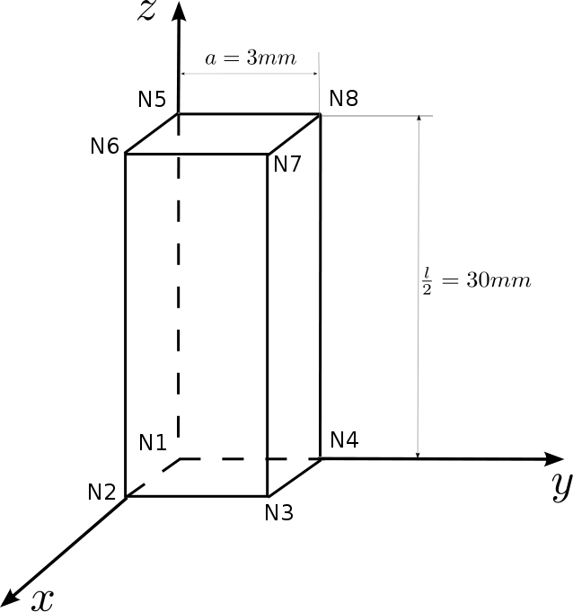
Figure 3.2-1: Modeling A mesh

3.3. Tested sizes and results

Two calculations are performed, the first with an explicit integration algorithm (ALGO_INTE =” RUNGE_KUTTA “), the second with an implicit integration algorithm (ALGO_INTE =” NEWTON”).

Calculation in explicit resolution:

Evolution of the constraint, \({\mathrm{\sigma }}_{0}\), as a function of time. This value is tested at various times:

Instant	Reference Type	Reference	Tolerance (%)
20	“ANALYTIQUE”	252.76091	0.5
2000	“ANALYTIQUE”	164.261	0.5
200000	“ANALYTIQUE”	101.596	0.5
1000000	“ANALYTIQUE”	75.97849999999999997	0.5
1600000	“ANALYTIQUE”	55.54209999999999998	10.0

Table 3.3-1 : Results of modeling A

Evolution of the damage variable, \(D\) as a function of time. This value is tested at various times depending on the modeling:

Instant	Reference Type	Reference	Tolerance (%)
20	“ANALYTIQUE”	2.3168400000000001E-4	0.5
2000	“ANALYTIQUE”	2.77144E-3	0.5
200000	“ANALYTIQUE”	0.032255100000000002	0.5
1000000	“ANALYTIQUE”	0.110134	1.0
1600000	“ANALYTIQUE”	0.28131600000000001	10.0

Table 3.3-2 : Results of modeling A

Evolution of the viscoplastic isotropic work hardening variable, \(r\), as a function of time. This value is tested at various times:

Instant	Reference Type	Reference	Tolerance (%)
20	“ANALYTIQUE”	1.6445100000000001E-3	0.5
2000	“ANALYTIQUE”	2.2312600000000001E-3	0.5
200000	“ANALYTIQUE”	2.6251500000000001E-3	0.5
1000000	“ANALYTIQUE”	2.747799999999999999E-3	0.5
1600000	“ANALYTIQUE”	2.79276E-3	0.5

Table 3.3-3 : Results of modeling A

Evolution of the viscoplastic isotropic work hardening variable, \(p\), as a function of time. This value is tested at various times:

Instant	Reference Type	Reference	Tolerance (%)
20	“ANALYTIQUE”	1.644569999999999999E-3	0.5
2000	“ANALYTIQUE”	2.231879999999999999E-3	0.5
200000	“ANALYTIQUE”	2.6301200000000001E-3	0.5
1000000	“ANALYTIQUE”	2.7607899999999999E-3	0.5
1600000	“ANALYTIQUE”	2.814779999999999998E-3	0.5

Table 3.3-4 : Results of modeling A

Calculation in resolution implicit :

Evolution of the constraint, \({\sigma }_{0}\), as a function of time. This value is tested at various times:

Instant	Reference Type	Reference	Tolerance (%)
20	“ANALYTIQUE”	252.76091	2.5
2000	“ANALYTIQUE”	164.261	2.5
200000	“ANALYTIQUE”	101.596	2.5

Table 3.3-5: Results of modeling A

Evolution of the damage variable, \(D\) as a function of time. This value is tested at various times depending on the modeling:

Instant	Reference Type	Reference	Tolerance (%)
20	“ANALYTIQUE”	2.3168400000000001E-4	3.5
2000	“ANALYTIQUE”	2.77144E-3	4.0
200000	“ANALYTIQUE”	0.032255100000000002	7.0

Table 3.3-6: Results of modeling A

Evolution of the viscoplastic isotropic work hardening variable, \(r\), as a function of time. This value is tested at various times:

Instant	Reference Type	Reference	Tolerance (%)
20	“ANALYTIQUE”	1.6445100000000001E-3	2.5
2000	“ANALYTIQUE”	2.2312600000000001E-3	1.0
200000	“ANALYTIQUE”	2.6251500000000001E-3	1.0

Table 3.3-7: Results of modeling A

Evolution of the viscoplastic isotropic work hardening variable, \(p\), as a function of time. This value is tested at various times:

Instant	Reference Type	Reference	Tolerance (%)
20	“ANALYTIQUE”	1.644569999999999999E-3	2.5
2000	“ANALYTIQUE”	2.231879999999999999E-3	1.0
200000	“ANALYTIQUE”	2.6301200000000001E-3	0.5

Table 3.3-8: Results of modeling A

Note: This calculation does not converge beyond the instant 200000.