5. C modeling#
5.1. Characteristics of modeling#
3D modeling is used.
Two calculations are performed that differ only in the integration algorithm: “NEWTON” and “RUNGE_KUTTA”.
In this case, the coefficient \({K}_{D}\) is chosen only depending on the temperature.
T (°C) |
900 |
1000 |
1025 |
\({K}_{D}\) |
15 |
15 |
15 |
Table 5.1-1 : K_D of C modeling
The discretization in time is quite fine:
(JUSQU_A = 2, NOMBRE = 10),

(JUSQU_A = 2., NOMBRE = 10),

(JUSQU_A = 20., NOMBRE = 10),

(JUSQU_A = 200., NOMBRE = 10),

(JUSQU_A = 2000., NOMBRE = 10),

(JUSQU_A = 20000., NOMBRE = 10),

(JUSQU_A = 200,000., NOMBRE = 10),

(JUSQU_A = 1000000., NOMBRE = 30),

(JUSQU_A = 1600000., NOMBRE = 30),

(JUSQU_A = 1700000., NOMBRE = 40),

(JUSQU_A = 1800000., NOMBRE = 40),

(JUSQU_A = 1900000., NOMBRE = 40),

(JUSQU_A = 2000000., NOMBRE = 40),

(JUSQU_A = 2100000., NOMBRE = 40),

(JUSQU_A = 2200000., NOMBRE = 40),

(JUSQU_A = 2300000., NOMBRE = 40),

(JUSQU_A = 2400000., NOMBRE = 40),

(JUSQU_A = 2500000., NOMBRE = 40),
5.2. Characteristics of the mesh#
It is chosen to represent the cylindrical test piece by a block in order to be able to perform a calculation on a single element. The modeling has 3 planes of symmetry.
Number of knots: 8
Number of stitches: 1 (HEXA8)
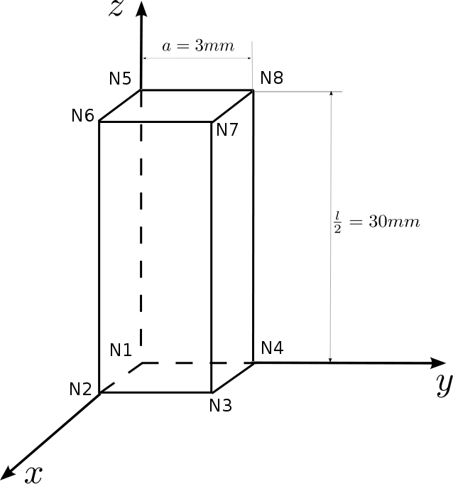
Figure 5.2-1: C modeling mesh
5.3. Tested sizes and results#
5.3.1. Case RUNGE_KUTTA + Matrix ELASTIQUE#
Evolution of the constraint, \({\sigma }_{0}\), as a function of time. This value is tested at various times:
Instant |
Reference Type |
Reference |
Tolerance (%) |
20 |
“ANALYTIQUE” |
253.02000000000001 |
0.5 |
2000 |
“ANALYTIQUE” |
164.36000000000001 |
0.5 |
200000 |
“ANALYTIQUE” |
102.16 |
0.5 |
1000000 |
“ANALYTIQUE” |
79.920000000000002 |
0.5 |
1600000 |
“ANALYTIQUE” |
70.900000000000006 |
1.0 |
Table 5.3.1-1 : C modeling results
Evolution of the damage variable, \(D\) as a function of time. This value is tested at various times depending on the modeling:
Instant |
Reference Type |
Reference |
Tolerance (%) |
20 |
“ANALYTIQUE” |
2.32E-4 |
0.5 |
2000 |
“ANALYTIQUE” |
2.7399E-3 |
0.5 |
200000 |
“ANALYTIQUE” |
0.027560999999999999 |
0.5 |
1000000 |
“ANALYTIQUE” |
0.066266500000000006 |
1.0 |
1600000 |
“ANALYTIQUE” |
0.090278800000000006 |
1.0 |
Table 5.3.1-2 : C modeling results
Evolution of the viscoplastic isotropic work hardening variable, \(r\), as a function of time. This value is tested at various times:
Instant |
Reference Type |
Reference |
Tolerance (%) |
20 |
“ANALYTIQUE” |
1.645999999999999999E-3 |
0.5 |
2000 |
“ANALYTIQUE” |
2.2339E-3 |
0.5 |
200000 |
“ANALYTIQUE” |
2.6282800000000002E-3 |
0.5 |
1000000 |
“ANALYTIQUE” |
2.7522900000000001E-3 |
0.5 |
1600000 |
“ANALYTIQUE” |
2.799299999999999998E-3 |
0.5 |
Table 5.3.1-3 : C modeling results
Evolution of the isotropic visco-plastic work hardening variable, \(p\), as a function of time. This value is tested at various times:
Instant |
Reference Type |
Reference |
Tolerance (%) |
20 |
“ANALYTIQUE” |
1.6461E-3 |
0.5 |
2000 |
“ANALYTIQUE” |
2.234499999999999999E-3 |
0.5 |
200000 |
“ANALYTIQUE” |
2.6329000000000001E-3 |
0.5 |
1000000 |
“ANALYTIQUE” |
2.762699E-3 |
0.5 |
1600000 |
“ANALYTIQUE” |
2.8137000000000001E-3 |
0.5 |
Table 5.3.1-4 : C modeling results
5.3.2. Case NEWTON + Matrix TANGENTE#
The quantities tested are the same as in the previous case. On the other hand, the tolerance is 4% (for all values tested).