7. F modeling#
7.1. Characteristics of modeling#
We use a AXIS model. Four calculations are performed with different matching options or contact algorithms.
7.2. Characteristics of the mesh#
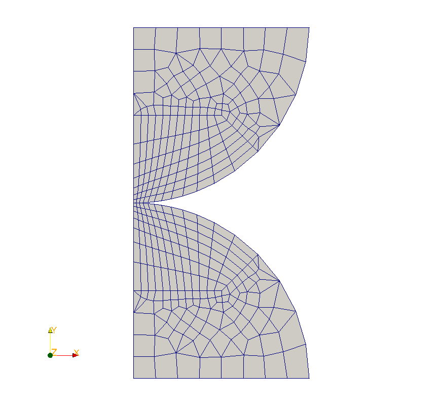
Knots: 376 knots.
Meshes: 30 TRIA3 and 324 QUAD4.
7.3. Tested sizes and results#
First calculation (nodal pairing, master-slave normal and algorithm “PENALISATION”)
Identification |
Reference type |
Reference value |
Tolerance |
mesh \(\mathit{M31}\) knot \(\mathit{N291}(G)\) |
“ANALYTIQUE” |
-2798.3 \(N\) |
7.0% |
\(\mathrm{DX}\) knot \(\mathit{N291}(G)\) |
“ANALYTIQUE” |
0 \(\mathit{mm}\) |
1.0E-10 |
\(\mathrm{DX}\) knot \(\mathit{N287}(H)\) |
“NON_REGRESSION” |
-0,110211 \(\mathit{mm}\) |
|
\(\mathrm{DY}\) knot \(\mathit{N287}(H)\) |
“NON_REGRESSION” |
-0,162912 \(\mathit{mm}\) |
|
\(\mathrm{DX}\) knot \(\mathit{N285}(I)\) |
“NON_REGRESSION” |
-0,165946 \(\mathit{mm}\) |
|
\(\mathrm{DY}\) knot \(\mathit{N285}(I)\) |
“NON_REGRESSION” |
-0.629667 \(\mathit{mm}\) |
Second calculation (normal master-slave, algorithm “PENALISATION”)
Identification |
Reference type |
Reference value |
Tolerance |
mesh \(\mathit{M31}\) knot \(\mathit{N291}(G)\) |
“ANALYTIQUE” |
-2798.3 \(N\) |
7.0% |
\(\mathrm{DX}\) knot \(\mathit{N291}(G)\) |
“ANALYTIQUE” |
0 \(\mathit{mm}\) |
1.0E-10 |
\(\mathrm{DX}\) knot \(\mathit{N287}(H)\) |
“NON_REGRESSION” |
-0,110678 \(\mathit{mm}\) |
|
\(\mathrm{DY}\) knot \(\mathit{N287}(H)\) |
“NON_REGRESSION” |
-0,162865 \(\mathit{mm}\) |
|
\(\mathrm{DX}\) knot \(\mathit{N285}(I)\) |
“NON_REGRESSION” |
-0,167194 \(\mathit{mm}\) |
|
\(\mathrm{DY}\) knot \(\mathit{N285}(I)\) |
“NON_REGRESSION” |
-0.628961 \(\mathit{mm}\) |
Third calculation (normal master-slave, algorithm “CONTRAINTE”)
Identification |
Reference type |
Reference value |
Tolerance |
mesh \(\mathit{M31}\) knot \(\mathit{N291}(G)\) |
“ANALYTIQUE” |
-2798.3 \(N\) |
7.0% |
\(\mathrm{DX}\) knot \(\mathit{N291}(G)\) |
“ANALYTIQUE” |
0 \(\mathit{mm}\) |
1.0E-10 |
\(\mathrm{DX}\) knot \(\mathit{N287}(H)\) |
“NON_REGRESSION” |
-0,110678 \(\mathit{mm}\) |
|
\(\mathrm{DY}\) knot \(\mathit{N287}(H)\) |
“NON_REGRESSION” |
-0,162901 \(\mathit{mm}\) |
|
\(\mathrm{DX}\) knot \(\mathit{N285}(I)\) |
“NON_REGRESSION” |
-0,167194 \(\mathit{mm}\) |
|
\(\mathrm{DY}\) knot \(\mathit{N285}(I)\) |
“NON_REGRESSION” |
-0.628947 \(\mathit{mm}\) |
Fourth calculation (smoothing, master-slave normal and algorithm “CONTRAINTE”)
Identification |
Reference type |
Reference value |
Tolerance |
mesh \(\mathit{M31}\) knot \(\mathit{N291}(G)\) |
“ANALYTIQUE” |
-2798.3 \(N\) |
7.0% |
\(\mathrm{DX}\) knot \(\mathit{N291}(G)\) |
“ANALYTIQUE” |
0 \(\mathit{mm}\) |
1.0E-10 |
\(\mathrm{DX}\) knot \(\mathit{N287}(H)\) |
“NON_REGRESSION” |
-0,110211 \(\mathit{mm}\) |
|
\(\mathrm{DY}\) knot \(\mathit{N287}(H)\) |
“NON_REGRESSION” |
-0,162911 \(\mathit{mm}\) |
|
\(\mathrm{DX}\) knot \(\mathit{N285}(I)\) |
“NON_REGRESSION” |
-0,165946 \(\mathit{mm}\) |
|
\(\mathrm{DY}\) knot \(\mathit{N285}(I)\) |
“NON_REGRESSION” |
-0.629666 \(\mathit{mm}\) |
7.4. notes#
On this modeling, we note that smoothing makes it possible to regain the symmetry of the problem (nodes perfectly facing each other once contact has been established), the last calculation in fact obtaining the same results as in nodal matching.
The values obtained are in good general agreement with the analytical solutions.