4. B modeling#
4.1. Characteristics of modeling#
We use a AXIS model. Three calculations are performed with different matching options or contact algorithms.
4.2. Characteristics of the mesh#
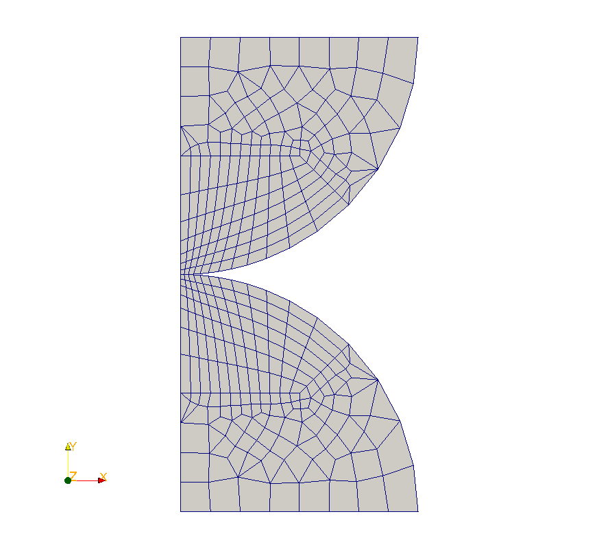
Knots: 376 knots.
Meshes: 30 TRIA3 and 324 QUAD4.
4.3. Tested sizes and results#
First calculation (algorithm “PENALISATION”, nodal matching, normal slave)
Identification |
Reference type |
Reference value |
Tolerance |
mesh \(\mathit{M31}\) knot \(\mathit{N291}(G)\) |
“ANALYTIQUE” |
-2798.3 \(N\) |
7.0% |
\(\mathrm{DX}\) knot \(\mathit{N291}(G)\) |
“ANALYTIQUE” |
0 \(\mathit{mm}\) |
1.0E-10 |
\(\mathrm{DX}\) knot \(\mathit{N287}(H)\) |
“NON_REGRESSION” |
-0,111338 \(\mathit{mm}\) |
|
\(\mathrm{DY}\) knot \(\mathit{N287}(H)\) |
“NON_REGRESSION” |
-0,161811 \(\mathit{mm}\) |
|
\(\mathrm{DX}\) knot \(\mathit{N285}(I)\) |
“NON_REGRESSION” |
-0,168635 \(\mathit{mm}\) |
|
\(\mathrm{DY}\) knot \(\mathit{N285}(I)\) |
“NON_REGRESSION” |
-0.628585 \(\mathit{mm}\) |
Second calculation (algorithm “PENALISATION”)
Identification |
Reference type |
Reference value |
Tolerance |
mesh \(\mathit{M31}\) knot \(\mathit{N291}(G)\) |
“ANALYTIQUE” |
-2798.3 \(N\) |
7.0% |
\(\mathrm{DX}\) knot \(\mathit{N291}(G)\) |
“ANALYTIQUE” |
0 \(\mathit{mm}\) |
1.0E-10 |
\(\mathrm{DX}\) knot \(\mathit{N287}(H)\) |
“NON_REGRESSION” |
-0.108104 \(\mathit{mm}\) |
|
\(\mathrm{DY}\) knot \(\mathit{N287}(H)\) |
“NON_REGRESSION” |
-0,164375 \(\mathit{mm}\) |
|
\(\mathrm{DX}\) knot \(\mathit{N285}(I)\) |
“NON_REGRESSION” |
-0,160912 \(\mathit{mm}\) |
|
\(\mathrm{DY}\) knot \(\mathit{N285}(I)\) |
“NON_REGRESSION” |
-0.631411 \(\mathit{mm}\) |
Third calculation (algorithm “CONTRAINTE”)
Identification |
Reference type |
Reference value |
Tolerance |
mesh \(\mathit{M31}\) knot \(\mathit{N291}(G)\) |
“ANALYTIQUE” |
-2798.3 \(N\) |
7.0% |
\(\mathrm{DX}\) knot \(\mathit{N291}(G)\) |
“ANALYTIQUE” |
0 \(\mathit{mm}\) |
1.0E-10 |
\(\mathrm{DX}\) knot \(\mathit{N287}(H)\) |
“NON_REGRESSION” |
-0.108104 \(\mathit{mm}\) |
|
\(\mathrm{DY}\) knot \(\mathit{N287}(H)\) |
“NON_REGRESSION” |
-0,164375 \(\mathit{mm}\) |
|
\(\mathrm{DX}\) knot \(\mathit{N285}(I)\) |
“NON_REGRESSION” |
-0,160912 \(\mathit{mm}\) |
|
\(\mathrm{DY}\) knot \(\mathit{N285}(I)\) |
“NON_REGRESSION” |
-0.631409 \(\mathit{mm}\) |
4.4. notes#
The difference between the contact pressure at point \(G\) and the analytical solution is explained on the one hand by extrapolation (passage from Gauss points to nodes) and on the other hand by the poor refinement of the mesh.
We note that the contact algorithms” PENALISATION “and” CONTRAINTE “give exactly the same results and that the nodal matching makes it possible to maintain the symmetry of the problem while giving results that are very similar to the node-facet pairing.