3. Modeling A#
3.1. Characteristics of modeling#
3D modeling is used. Because of symmetry, only one quarter of a hemisphere is represented, a condition such as a unilateral link makes it possible to complete the modeling.
In this modeling, the points \(H\) and \({H}_{p}\) (respectively \(I\) and \({I}_{p}\)) (respectively and) are the same points (with respect to those described in the geometry) but located on the two faces supporting the symmetry conditions.
The results obtained with this modeling serve as a reference (AUTRE_ASTER) for the three-dimensional I and J models.
3.2. Characteristics of the mesh#
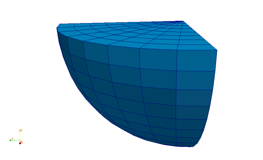
Knots: 1849.
Meshes: 96 TETRA4, 2936 PENTA6, 112 PYRAM5.
3.3. Tested sizes and results#
First calculation (formulation “LIAISON_UNIL”)
Identification |
Reference type |
Reference value |
Tolerance |
mesh \(\mathit{M2948}\) stitch \(G\) |
“ANALYTIQUE” |
-2798.3 \(N\) |
14.0% |
mesh \(\mathit{M2948}\) stitch \(G\) |
“NON_REGRESSION” |
-3176.3 \(N\) |
1.0% -4% |
mesh \(\mathit{M2960}\) stitch \(G\) |
“NON_REGRESSION” |
-3176.3 \(N\) |
1.0% -4% |
mesh \(\mathit{M2972}\) stitch \(G\) |
“NON_REGRESSION” |
-3176.3 \(N\) |
1.0% -4% |
mesh \(\mathit{M2984}\) stitch \(G\) |
“NON_REGRESSION” |
-3176.3 \(N\) |
1.0% -4% |
mesh \(\mathit{M2996}\) stitch \(G\) |
“NON_REGRESSION” |
-3176.3 \(N\) |
1.0% -4% |
mesh \(\mathit{M3008}\) stitch \(G\) |
“NON_REGRESSION” |
-3176.3 \(N\) |
1.0% -4% |
mesh \(\mathit{M3020}\) stitch \(G\) |
“NON_REGRESSION” |
-3176.3 \(N\) |
1.0% -4% |
mesh \(\mathit{M3032}\) stitch \(G\) |
“NON_REGRESSION” |
-3176.3 \(N\) |
1.0% -4% |
\(\mathit{DX}\) point \(G\) |
“ANALYTIQUE” |
0 \(\mathit{mm}\) |
1.0E-10 |
\(\mathit{DX}\) point \(H\) |
“NON_REGRESSION” |
-0,11343 \(\mathit{mm}\) |
1.0% -4% |
\(\mathit{DZ}\) point \({H}_{p}\) |
“NON_REGRESSION” |
-0,11343 \(\mathit{mm}\) |
1.0% -4% |
\(\mathit{DY}\) point \(H\) |
“NON_REGRESSION” |
-0,16291 \(\mathit{mm}\) |
1.0% -4% |
\(\mathit{DY}\) point \({H}_{p}\) |
“NON_REGRESSION” |
-0,16291 \(\mathit{mm}\) |
1.0% -4% |
\(\mathit{DX}\) point \(I\) |
“NON_REGRESSION” |
-0,17845 \(\mathit{mm}\) |
1.0% -4% |
\(\mathit{DZ}\) point \({I}_{p}\) |
“NON_REGRESSION” |
-0,17845 \(\mathit{mm}\) |
1.0% -4% |
\(\mathit{DY}\) point \(I\) |
“NON_REGRESSION” |
-0.62966 \(\mathit{mm}\) |
1.0% -4% |
\(\mathit{DY}\) point \({I}_{p}\) |
“NON_REGRESSION” |
-0.62966 \(\mathit{mm}\) |
1.0% -4% |
3.4. notes#
The results obtained in this three-dimensional modeling are in good agreement with the analytical solution. It is also noted that the radiating mesh makes it possible to maintain the axisymmetry of the problem, which is why the results obtained in each mesh that contributes to point \(G\) are similar.
This modeling validates the use of a unilateral condition that is a function of space, i.e. whose « game » is not the same for all constrained nodes. The results obtained are identical to contact modeling.