1. Reference problem#
1.1. Geometry#
Structure \(\mathrm{2D}\) is a rectangular plate (\(\mathrm{LX}=\mathrm{0,2}m\), \(\mathrm{LY}=\mathrm{0,5}m\)), with a right central crack, inclined at a variable angle \(\theta\) with respect to the horizontal axis [Figure 1.1-1]. The crack length is constant (\(a=\mathrm{0,04}m\)). In this test, the angle \(\theta\) will successively take the values: \(0°\), \(15°\),, \(30°\),, \(45°\), \(60°\) for modeling \(A\) and \(0°\), \(45°\) for modeling \(B\).
We call the « bottom line » the line in \(y=-\mathrm{LY}/2\) and « top line » the line in \(y=\mathrm{LY}/2\).
The nodes marked \(A\), \(B\), \(C\), and \(D\) on the Figure 1.1-1 serve to impose boundary conditions, which are explained in paragraph [§ 1.3].
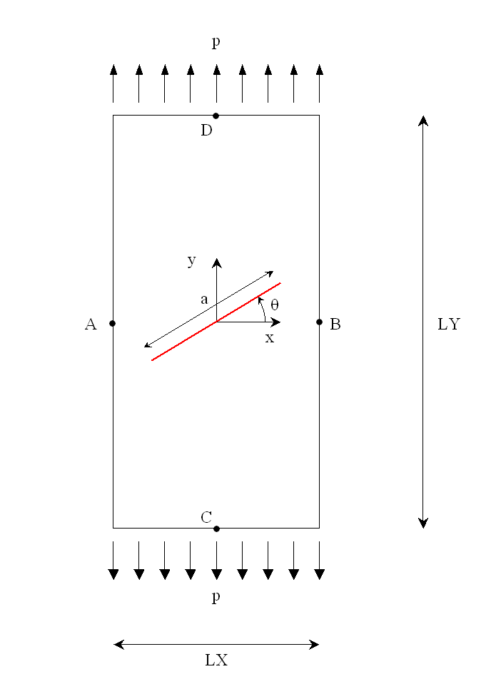
Figure 1.1-1 : geometry of the cracked plate and loading of the modelling \(A\) .
1.2. Material properties#
Young’s module: \(E=210{10}^{9}\mathrm{Pa}\)
Poisson’s ratio: modeling A \(\nu =0.3\), modeling B \(\nu =0\)
Density: B modeling: \(\rho =7800\mathrm{kg}/{m}^{3}\)
1.3. Boundary conditions and loads#
Modeling \(A\) :
Loading consists of applying a force distributed over the lower and upper lines \(p={10}^{6}\mathrm{Pa}\).
In order to block rigid modes, we block the movements of the nodes \(A\), \(B\), \(C\) and \(D\) as follows:
\({\mathrm{DY}}^{A}={\mathrm{DY}}^{B}=0\);
\({\mathrm{DX}}^{C}={\mathrm{DX}}^{D}=0\).
Modeling \(B\) :
Charging consists in applying to the plate an embedment on the upper line and a volume force of type FORCE_INTERNE or PESANTEUR. We make sure to apply the same load (following \(-Y\)) for two successive calculations with these key words: for the first imposed force density of \(78000N/{m}^{3}\) and for the second one chooses an acceleration due to gravity equal to \(10{\mathrm{m.s}}^{-2}\) and therefore a force density of \(10.\rho =78000N/{m}^{3}\).
Models \(C\) , \(D\) , , \(E\) :
Same assumptions as modeling \(A\)
Modeling \(F\) :
The tensile load on the upper and lower faces is replaced by pressure on the lips of the crack (the 2 loads are equivalent)
1.4. Benchmark solution#
Modeling \(A\) :
The analytic expressions for the stress intensity factors \({K}_{I}\) and \({K}_{\mathrm{II}}\) are functions of the distributed force \(p\), the crack length \(a\), the plate width \(\mathrm{LX}\), and the angle \(\theta\):
\(\begin{array}{}{K}_{I}=p\sqrt{\pi \frac{a}{2}}F(\frac{a}{\mathrm{Lx}})\mathrm{cos²}\theta \\ {K}_{\mathrm{II}}=p\sqrt{\pi \frac{a}{2}}F(\frac{a}{\mathrm{Lx}})\mathrm{cos}\theta \mathrm{sin}\theta \end{array}\)
where function \(F\) can be determined in several different ways. We choose the one obtained by Brown in 1966 [bib2, p41], whose precision is less than \(\text{0,5\%}\) if the ratio between the length of the crack and the width of the plate is less than or equal to \(\mathrm{0,7}\) (in our case, \(a/\mathrm{LX}=\mathrm{0,2}\)):
With the numerical values of the test:
Reference |
||
\(\alpha\) (°) |
\({K}_{I}({\mathit{Pa.m}}^{\mathrm{-}1\mathrm{/}2})\) |
\({K}_{\mathit{II}}({\mathit{Pa.m}}^{\mathrm{-}1\mathrm{/}2})\) |
0 |
2.5725024656 105 |
0 |
15 |
2,4001774761 105 |
6,4312561642 104 |
30 |
1.9293768492 105 |
1,1139262432 105 |
45 |
1,2862512328 105 |
1,2862512328 105 |
60 |
6,4312561641 104 |
1,1139262432 105 |
Table 1.4-1 : reference values for \({K}_{I}\) and \({K}_{\mathrm{II}}\)
Theoretically, these values are the same for both crack bottoms.
Modeling \(B\) :
Non-regression tests are carried out.
Models \(C\) , \(D\) , , \(E\) , \(F\) :
We use the reference values from modeling \(A\)
1.5. Bibliographical references#
GENIAUT S., MASSIN P.: eXtended Finite Element Method, Code_Aster Reference Manual, [R7.02.12]
TADA H., PARIS P., IRWIN G.:The stress analysis of cracks handbook, 3rd ed., 2000