2. Reference solutions#
2.1. Calculation method used for reference solutions#
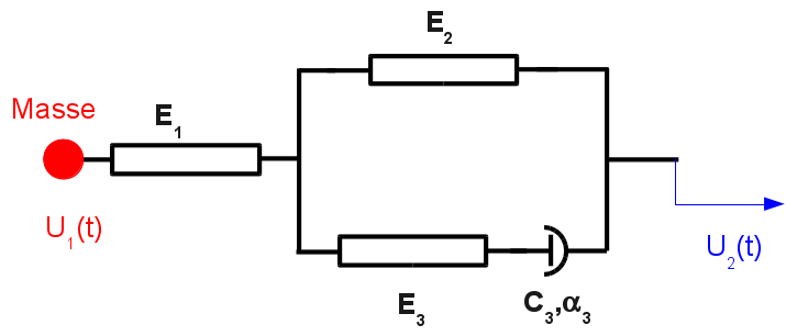
2.1.1. Modeling A#
This modeling compares a system of discretes (stiffness and linear damper, so \({\alpha }_{3}=1\)) assembled in series and in parallel to a discrete system affected by the law of behavior DIS_VISC. This comparison is carried out in linear transient dynamics by simulating a release test.
The equations of the differential system, which is of 3rd order, describing the analytical solution are:
\(\{\begin{array}{c}{F}_{1}=m\ddot{{U}_{1}}\\ {\dot{F}}_{1}.\left(\frac{1}{{E}_{1}}+\frac{1}{{E}_{3}}+\frac{{E}_{2}}{{E}_{1}.{E}_{3}}\right)=\left({\dot{U}}_{2}-{\dot{U}}_{1}\right)\left(1+\frac{{E}_{2}}{{E}_{3}}\right)-\frac{1}{{C}_{3}}.\left({F}_{1}.\left(1+\frac{{E}_{2}}{{E}_{1}}\right)-{E}_{2}.\left({U}_{2}-{U}_{1}\right)\right)\end{array}\) [éq2.1.1-1]
The initial conditions are, with \({U}_{0}=\mathrm{0,1}m\):
\({\ddot{U}}_{1}(t=0)=0\) \({\dot{U}}_{1}(t=0)=0\) \({U}_{1}(t=0)=0\) \({U}_{2}(t)={U}_{0}.H(t)\mathit{avec}H\mathit{la}\mathit{fonction}\mathit{de}\mathit{Heaviside}\)
The numerical integration of this differential system is obtained with the Laplace transform technique:
\({U}_{1}(t)={A}_{s}\mathrm{exp}(-{\lambda }_{\mathit{sc}}t)\mathrm{sin}({\omega }_{t}t)-{A}_{c}\mathrm{exp}(-{\lambda }_{\mathit{sc}}t)\mathrm{cos}({\omega }_{t}t)+{A}_{e}\mathrm{exp}(-{\lambda }_{e}t)+\frac{1}{10}\) [éq2.1.1-2]
\({F}_{1}(t)=-{B}_{s}\mathrm{exp}(-{\lambda }_{\mathit{sc}}t)\mathrm{sin}({\omega }_{t}t)+{B}_{c}\mathrm{exp}(-{\lambda }_{\mathit{sc}}t)\mathrm{cos}({\omega }_{t}t)+{B}_{e}\mathrm{exp}(-{\lambda }_{e}t)\) [éq2.1.1-3]
With
\(\begin{array}{ccc}{\omega }_{t}=\frac{14593}{4792}{s}^{-1}& & \\ {A}_{s}=\frac{5516}{214807}& {\lambda }_{\mathit{sc}}=\frac{1573}{2072}{s}^{-1}& {B}_{s}=\frac{5625}{7831}\\ {A}_{c}=\frac{3137}{29305}& & {B}_{c}=\frac{9170}{11289}\\ {A}_{e}=\frac{413}{58610}& {\lambda }_{e}=\frac{38132}{1685}{s}^{-1}& {B}_{e}=\frac{12692}{3517}\end{array}\)
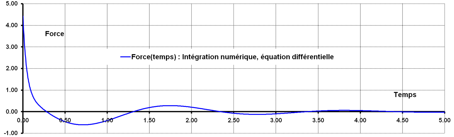
Figure 2.1.1-a : Evolution of effort as a function of time, modeling A.
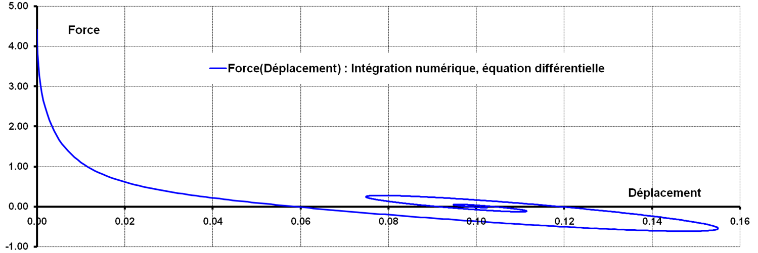
Figure 2.1.1-b : Evolution of effort as a function of displacement \({U}_{1}\) , modeling A.
2.1.2. B, C, D, E models#
The equations governing behavior are nonlinear differential equations. To validate the answer obtained with Code_Aster, an integration by a Runge-Kutta method is carried out with a tool external to Code_Aster.
Comparisons are made on the displacement and on the effort.
2.2. Uncertainty about the solution#
2.2.1. Modeling A#
For the effort response, displacement:
The reference solution is obtained by numerical integration of a differential system, using the Laplace transform technique. There is no uncertainty, the solution is analytical.
2.2.2. B, C, D, E models#
For the effort response, displacement:
The reference solution is obtained by numerical integration of a differential system.