1. Reference problem#
1.1. Device description#
The viscous damper is represented by the rheological model below.
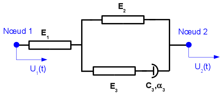
Figure 1.1-a: Rheological model of the viscous damper.
The values of the various stiffness \({E}_{1}\), \({E}_{2}\), \({E}_{3}\) and the characteristics of the non-linear viscous part \({C}_{3}\), \({\alpha }_{3}\) are derived from tests. The equations governing the behavior are [R5.03.17]:
\({\dot{F}}_{1}\left(\frac{1}{{E}_{1}}+\frac{1}{{E}_{3}}+\frac{{E}_{2}}{\left({E}_{1}.{E}_{3}\right)}\right)=\left({\dot{U}}_{2}-{\dot{U}}_{1}\right)\left(1+\frac{{E}_{2}}{{E}_{3}}\right)-{\langle \langle \frac{{F}_{1}}{{C}_{3}}\left(1+\frac{{E}_{2}}{{E}_{1}}\right)-\frac{{E}_{2}}{{C}_{3}}\left({U}_{2}-{U}_{1}\right)\rangle \rangle }^{1/{\alpha }_{3}}\)
with \(\begin{array}{cc}{\langle \langle x\rangle \rangle }^{a}={x}^{a}& \mathit{si}x\ge 0\\ {\langle \langle x\rangle \rangle }^{a}=-{∣x∣}^{a}& \mathit{si}x\le 0\end{array}\)
The dissipation increment is:
\(\Delta D={C}_{3}.{∣\frac{{F}_{1}}{{C}_{3}}\left(1+\frac{{E}_{2}}{{E}_{1}}\right)-\frac{{E}_{2}}{{C}_{3}}\left({U}_{2}-{U}_{1}\right)∣}^{1+1/{\alpha }_{3}}\)
1.2. Modellations#
Note: The units of the parameters must agree with the unit of effort, the unit of length, and the unit of time of the problem [R5.03.17]. For all models the units are homogeneous to [N], [m], [s].
1.2.1. Modeling A#
This modeling compares a system of discretes (stiffness and linear damper) assembled in series and in parallel to a discrete affected by the law of behavior DIS_VISC, with \({\alpha }_{3}=1\), and a point mass \(m=1.0\mathit{kg}\). This comparison is carried out in transient linear dynamics by simulating a release test.
1.2.2. B, C, D, E models#
This modeling is carried out in non-linear dynamics and simulates the loading due to an earthquake. The acceleration is sinusoidal for 4 periods, then zero acceleration. The CALC_CHAR_SEISME command allows you to define the solicitation.
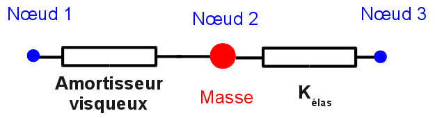
Figure 1.2.2-a : Model system.
Modeling B is carried out with the operator DYNA_NON_LINE. The C, D, E models are carried out with the operator DYNA_VIBRA (TYPE_CALCUL =” TRAN “, =””, BASE_CALCUL =” GENE “) equivalent to the command DYNA_TRAN_MODAL, with a time diagram of the type Euler, Runge-Kutta of order 5 and Runge-Kutta of order 5 and Runge-Kutta of order 3, respectively.
1.3. Material properties#
1.3.1. Modeling A#
The characteristics of the shock absorber are:
\(\mathit{K1}=120.0\), \(\mathit{K2}=10.0\), \(\mathit{K3}=60.0\), \(C=1.7\), \(\mathit{PUIS}\text{\_}\mathit{ALPHA}=1.0\)
The mass value is \(m=1.0\mathit{kg}\).
1.3.2. B modeling#
The characteristics of the shock absorber are:
\(\mathit{K1}=120.0\), \(\mathit{K2}=10.0\), \(\mathit{K3}=60.0\), \(C=1.7\), \(\mathit{PUIS}\text{\_}\mathit{ALPHA}=0.50\)
The spring stiffness is \(k=1.0{\mathit{N.m}}^{-1}\), the mass is \(m=1.0\mathit{kg}\).
1.3.3. C, D, E modeling#
The characteristics of the shock absorber are given under the keyword DIS_VISC of the DYNA_VIBRA or DYNA_TRAN_MODAL command.
\(\mathit{K1}=120.0\), \(\mathit{K2}=10.0\), \(\mathit{K3}=60.0\), \(C=1.7\), \(\mathit{PUIS}\text{\_}\mathit{ALPHA}=0.50\)
The spring stiffness is \(k=1.0{\mathit{N.m}}^{-1}\), the mass is \(m=1.0\mathit{kg}\).
1.4. Boundary conditions and loads#
When the discrete is a SEG2, one of the nodes is blocked, on the other a displacement condition is imposed. When the discrete is a POI1 the displacement condition is imposed on this node.
In modeling A, the displacement is imposed and remains constant: \({U}_{0}=0.1\)
The on-the-go condition is a function of time for B, C, D, and E models:
\({U}_{0}.\mathrm{sin}(2\pi .\mathit{f.t})\) with \(f=5\mathit{Hz}\) for 4 periods, then \(0\).