3. Modeling A#
M266 ROAD
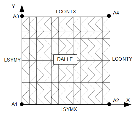
3.1. Characteristics of the mesh#
Number of knots: 169
Number of meshes and type: 288 TRIA3
3.2. Tested sizes and results#
Identification |
Reference Type |
Reference |
Tolerance (%) |
\(\mathrm{DZ}(\mathrm{A1})\) |
“ANALYTIQUE” |
2.433 10-4 |
|
\(\mathrm{MXX}(\mathrm{A1})\) |
“ANALYTIQUE” |
|
|
\(\mathrm{KXX}(\mathrm{A1})\) |
“ANALYTIQUE” |
7.21 10-4 |
|
Identification |
Reference type |
Reference |
Tolerance (%) |
||
\(\mathit{MXX}\) |
\(\mathit{M266}\) |
\(\mathit{Point}3\) |
“NON_REGRESSION” |
4044.16 |
1.e-6 |
\(\mathit{KXX}\) |
\(\mathit{M266}\) |
\(\mathit{Point}3\) |
“NON_REGRESSION” |
7.1996 10-4 |
1.e-6 |
The quantities are expressed in the coordinate system defined by the nautical angles \(\alpha \mathrm{=}33°\) and \(\beta \mathrm{=}12°\).
Identification |
Reference Type |
Reference |
Tolerance (%) |
\(\mathrm{DZ}(\mathrm{A1})\) |
“ANALYTIQUE” |
2.433 10-4 |
|
\(\mathit{MXX}(\mathit{A1})\) |
“NON_REGRESSION” |
2847.47 |
1.e-6 |
\(\mathit{MYY}(\mathit{A1})\) |
“NON_REGRESSION” |
1198.15 |
1.e-6 |
\(\mathit{MXY}(\mathit{A1})\) |
“NON_REGRESSION” |
-1852.21 |
1.e-6 |
\(\mathit{KXX}(\mathit{A1})\) |
“NON_REGRESSION” |
5.0692 10-4 |
1.e-6 |
\(\mathit{KYY}(\mathit{A1})\) |
“NON_REGRESSION” |
2.1330 10-4 |
1.e-6 |
\(\mathit{KXY}(\mathit{A1})\) |
“NON_REGRESSION” |
-3.2974 10-4 |
1.e-6 |
Identification |
Reference type |
Reference |
Tolerance (%) |
||
\(\mathit{MXX}\) |
\(\mathit{M266}\) |
\(\mathit{Point}3\) |
“NON_REGRESSION” |
2842.56 |
1.e-6 |
\(\mathit{MYY}\) |
\(\mathit{M266}\) |
\(\mathit{Point}3\) |
“NON_REGRESSION” |
1197.70 |
1.e-6 |
\(\mathit{MXY}\) |
\(\mathit{M266}\) |
\(\mathit{Point}3\) |
“NON_REGRESSION” |
-1849.40 |
1.e-6 |
\(\mathit{KXX}\) |
\(\mathit{M266}\) |
\(\mathit{Point}3\) |
“NON_REGRESSION” |
5.0605 10-4 |
1.e-6 |
\(\mathit{KYY}\) |
\(\mathit{M266}\) |
\(\mathit{Point}3\) |
“NON_REGRESSION” |
2.1322 10-4 |
1.e-6 |
\(\mathit{KXY}\) |
\(\mathit{M266}\) |
\(\mathit{Point}3\) |
“NON_REGRESSION” |
-3.2924 10-4 |
1.e-6 |
3.3. notes#
The coefficients of the following elasticity matrices, used during the calculations, were calculated with \({\nu }_{b}=0\):
Membrane elasticity matrix: \(\left\{\begin{array}{ccc}4614.& 0& 0\\ 0& 4614.& 0\\ 0& 0& 2142.\end{array}\right\}{10}^{6}N\mathrm{/}m\)
Flexural elasticity matrix: \(\left\{\begin{array}{ccc}5.617& 0& 0\\ 0& 5.617& 0\\ 0& 0& 2.57\end{array}\right\}{10}^{6}N/m\)
To be certain of staying within the elastic domain, the elastic limits, expressed in the orthotropy coordinate system, are set arbitrarily to a very high value:
Elastic limits in positive flexure:
Direction \(x\): \({1.10}^{10}\mathrm{MNm}/\mathrm{ml}\)
Direction \(y\): \({1.10}^{10}\mathrm{MNm}/\mathrm{ml}\)
Elastic limits in negative flexure:
Direction \(x\): \(–{1.10}^{10}\mathrm{MNm}/\mathrm{ml}\)
Direction \(y\): \(–{1.10}^{10}\mathrm{MNm}/\mathrm{ml}\)
As the structure remains in the elastic domain, the kinematic recall coefficient (Prager constant) can take any value.