1. Reference problem#
1.1. Geometry#
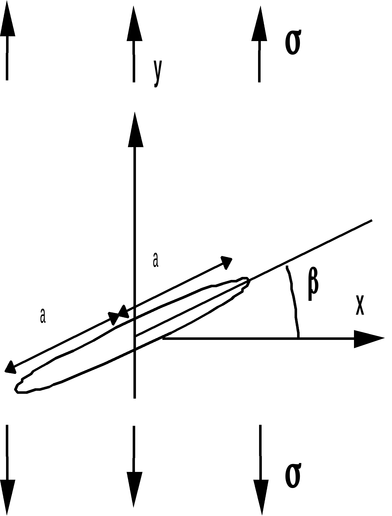
We assign any value to the inclination, \(\beta \mathrm{=}37\mathit{degrés}\).
We choose \(a=1.E-3m\).
1.2. Material properties#
The material is isotropic linear elastic, with a Young’s modulus \(E=2.E11\mathrm{Pa}\) and a Poisson’s ratio \(\nu =0.3\).
The traction curve is defined as:
the slope is equal to 3.
the elastic limit is equal to \(1.88\mathrm{GPa}\).
The hypothesis of plane constraints is applied.
1.3. Boundary conditions and loads#
Arbitrary mesh domain limits:
\(-{x}_{\mathrm{max}}\le x\le {x}_{\mathrm{max}}\) with \({x}_{\mathrm{max}}=\mathrm{10a}\)
\(-{y}_{\mathrm{max}}\le y\le {y}_{\mathrm{max}}\) with \({y}_{\mathrm{max}}=\mathrm{20a}\)
Boundary conditions:
In order to exclusively block the 3 rigid plane modes.
\(\mathrm{UX}=\mathrm{UY}=0\) at the bottom left corner of the full model.
\(\mathrm{UY}=0\) at the bottom right corner of the full model.
On the bottom edge, we impose \(\mathrm{UY}=0\)
Charging: uniform tension \({\sigma }_{\mathrm{yy}}={\sigma }_{0}\) on the top edge:
The value of \({\sigma }_{0}\) is \(\mathrm{100MPa}\), in plane constraints.