3. Modeling A

3.1. Characteristics of modeling A

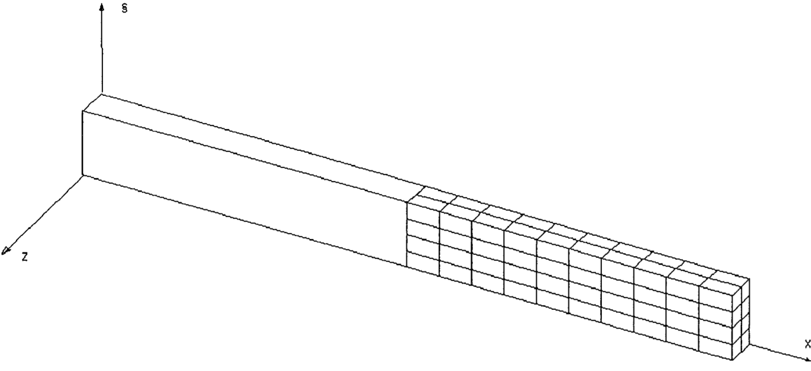
Figure 3.1 Meshing the geometry of the problem.

The beam is divided into two equal parts. Each half is represented by a substructure. These are generated using the Mac-Neal method.

3.2. Characteristics of the mesh

Number of knots: 557

Number of meshes and types: 80 HEXA20, 20 QUAD8

3.3. Tested sizes and results

Location	Quantity Type	Reference Value	Reference Type	Tolerance (%)
\(X=\frac{L}{4}\) (first half)	\(\mathit{DY}\)	\(1.95994\times {10}^{-5}+8.49179\times {10}^{-6}j\)		“ANALYTIQUE”	\(5.0\)
\(X=\frac{L}{2}\) (first half)	\(\mathit{DY}\)	\(-6.999387\times {10}^{-6}-1.14501\times {10}^{-5}j\)		“ANALYTIQUE”	\(5.0\)
\(X=\frac{L}{2}\) (second half)	\(\mathit{DY}\)	\(-6.999387\times {10}^{-6}-1.14501\times {10}^{-5}j\)		“ANALYTIQUE”	\(5.0\)
\(X=3\frac{L}{4}\) (second half)	\(\mathit{DY}\)	\(1.95994\times {10}^{-5}+8.49179\times {10}^{-6}j\)		“ANALYTIQUE”	\(5.0\)