1. Reference problem#
1.1. Geometry#
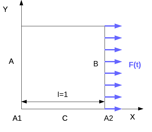
Square plate :
Length: \(l=1.0m\)
Thickness: \(e=0.1m\)
1.2. Material properties#
Young’s module, \(E=4.388{10}^{10}N/{m}^{2}\)
Poisson’s ratio, \(\nu =0.0\)
Density, \(\rho =2500.0\mathrm{kg}/{m}^{3}\)
1.3. Boundary conditions and loads#
Boundary conditions:
L location |
Blocked components |
A1 |
DX, DY, DZ, DRX, DRY, DRZ |
A |
DX, DZ, DRX, DRY, DRZ |
C |
DZ, DRX, DRY, DRZ |
Loads:
We apply the linear force on side B in the direction \(x\), which depends on time like,
\(F(t)={Q}_{0}EKe\mathrm{cos}(\mathrm{Kl})\mathrm{sin}(\omega t)\),
where the following parameters are used:
\({Q}_{0}\) (\(={10}^{-4}m\)) - load amplitude
\(E\) — Young’s modulus defined above (in \(N/{m}^{2}\))
\(e\) — the thickness defined above (in \(m\))
\(l\) — the plate size defined above (in \(m\))
\(K\) (\(=\frac{\pi }{\mathrm{8l}}\)) the wave number of the analytical solution (in \({m}^{-1}\))
\(\omega\) — frequency (times \(2\pi\)), linked to the wave number \(K\), \(K=\omega /c\), \(c\) being the speed of the waves in the structure, \(c=\sqrt{\frac{E}{\rho }}\)
The parameterization introduced makes it possible to apply the load just to obtain the analytical solution, determined simply by the parameters \({Q}_{0}\) and \(K\), and then by other parameters of the dimensions and material properties of the structure.
1.4. Initial conditions#
Initially, the movements are zero everywhere and the speeds obey the following spatial distribution,
\({v}_{0}(x,y)=\omega {Q}_{0}\mathrm{sin}(\mathrm{K.x})\)