1. Reference problem#
1.1. Geometry#
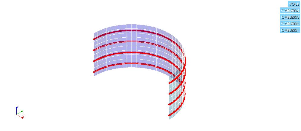
The concrete veil has a semi-cylindrical shape: the height is \(H=10m\) and the average radius is \(R\mathrm{=}\mathrm{10 }m\).
The thickness of the veil is \(e\mathrm{=}\mathrm{0,6}m\). The « equivalent mean radius », in the sense of BPEL on the vertical section of the veil is therefore equal to \({r}_{m}\mathrm{=}\mathrm{0,283}m\), knowing that:
\({r}_{m}\mathrm{=}\frac{\mathit{eH}}{2(e+H)}\) (reference BPEL 2.1.5)
The cables each describe a semicircle in a horizontal plane, and thus travel along the length of the veil. The dimensions of the plans containing the cables are:
for cable 1: \({z}_{1}\mathrm{=}1m\);
for cable no. 2: \({z}_{2}=\mathrm{3,5}m\);
for cable no. 3: \({z}_{3}=6m\);
for cable no. 4: \({z}_{4}=\mathrm{8,5}m\).
The cables 3 and 4 have an eccentricity with respect to the mean radius of the veil, equal respectively to:
\({\mathrm{ex}}_{3}=\mathrm{0,05}m\);
\({\mathrm{ex}}_{4}=\mathrm{0,1}m\).
The cross-sectional area of each cable is \({S}_{a}=\mathrm{1,5}{.10}^{-4}{m}^{2}\).
1.2. Material properties#
1.2.1. Material: concrete constituting the veil#
Elastic properties:
Young’s module |
\({E}_{b}={3.10}^{10}\mathrm{Pa}\) |
Poisson’s Ratio |
\({\nu }_{b}=\mathrm{0,2}\) |
Characteristic parameters for estimating voltage losses:
Flat rate of tension loss due to concrete creep |
\({x}_{\mathrm{flu}}=\mathrm{0,07}\) |
Flat rate of stress loss due to concrete shrinkage |
\({x}_{\mathrm{ret}}=\mathrm{0,08}\) |
1.2.2. Material: steel constituting the cables#
Elastic properties:
Young’s module |
\({E}_{a}=\mathrm{2,1}{.10}^{11}\mathrm{Pa}\) |
Poisson’s Ratio |
\({\nu }_{a}\mathrm{=}\mathrm{0,3}\) |
Characteristic parameters for estimating voltage losses: |
|
Relaxation of steel at 1000 hours |
\({\rho }_{1000}\mathrm{=}2\text{\%}\) |
Dimensional relaxation coefficient of prestressed steel |
\({\mu }_{0}\mathrm{=}\mathrm{0,3}\) |
Elastic limit stress of steel |
\({f}_{\mathit{prg}}\mathrm{=}\mathrm{1,77}{.10}^{9}\mathit{Pa}\) |
Curved friction coefficient |
\(f=\mathrm{0,2}{\mathrm{rad}}^{-1}\) |
Tension loss coefficient per unit length |
\(\varphi \mathrm{=}{3.10}^{\mathrm{-}3}{m}^{\mathrm{-}1}\) |
1.3. Loading#
A normal force of traction is applied to both ends of each cable. The value of the voltage applied is \({F}_{0}\mathrm{=}{2.10}^{5}N\).
To evaluate the voltage losses due to cable relaxation over time, the following relationships are used:
\(\Delta {\sigma }_{\mathit{pj}}\mathrm{=}\Delta {\sigma }_{p}(x)r(j)\) |
(reference BPEL 3.3,24) |
\(\Delta {\sigma }_{p}\mathrm{=}\frac{6}{100}{\rho }_{1000}(\frac{{\sigma }_{\mathit{pi}}(x)}{{f}_{\mathit{prg}}}\mathrm{-}{\mu }_{0}){\sigma }_{\mathit{pi}}(x)\) |
(reference BPEL 3.3,23) |
\(r(j)\mathrm{=}\frac{j}{j+9\mathrm{\times }{r}_{m}}\) |
(reference BPEL 3.3,24 and 2.1,51) |
\({\sigma }_{\mathit{pi}}(x)\) |
called initial voltage, the voltage at the \(x\) abscissa point, after instantaneous voltage losses. |
\(j\) |
evaluation moment, in days |
\({r}_{m}\) |
equivalent mean radius, in \(\mathit{cm}\) |
The characteristics are evaluated on day \(j\mathrm{=}10\).
To assess the voltage losses in the vicinity of the anchorages, a setback at anchors \(\Delta \mathrm{=}{5.10}^{\mathrm{-}4}m\) is taken into account.
Note:
This problem ignores the resolution of the balance of the complete steel-concrete structure and is limited to the determination according to the BPEL of the prestress in the cables.