2. Data creation/import#
This paragraph describes the « data » portion of Grace. There are three ways to get data to plot in Grace:
by importing data into files;
by creating data (via sampled mathematical functions);
by duplicating and modifying existing data.
2.1. Importing#
Grace is able to import curves from text files. These files should only contain data (except lines starting with # which are considered comment lines).
Data must be in columns (separated by spaces or tab characters). Attention, a file can only contain a single « data block », i.e. data on several columns and several rows (unlike the.dogr files previously used by the Agraf tool).
Grace can read the different columns in the form:
|
|
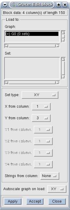
|
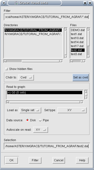
In practice, the import is done from the « Data/Import/Ascii… » menu, which opens the dialog window above. Note:
|
2.2. Data creation by mathematical function#
To define a curve, the following commands must be linked together:
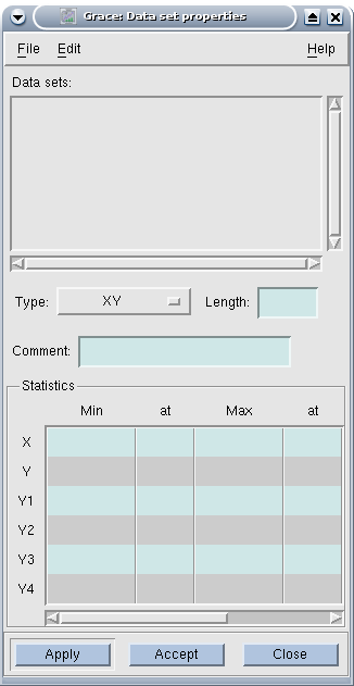
Edit/Data sets…
Right click in the area under « Data sets »;
Choose « Create New/By Formula », which opens the next box, which must be filled in. For example, to plot sin (x) +2.5 from -10 to 10 in 100 steps;
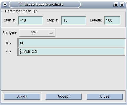
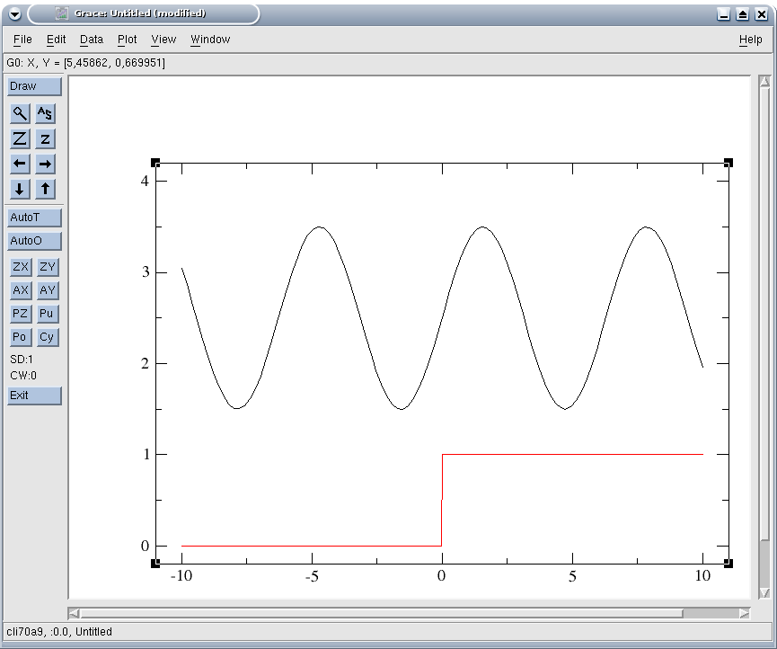
After « Accept » then « Close », possibly « Autoscale » button (tool (see paragraph [§5] detailing Grace’s toolbar) « AS » to the right of the zoom magnifying glass) to display the curve at the correct scale.
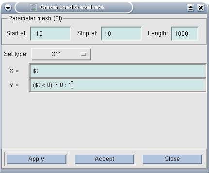
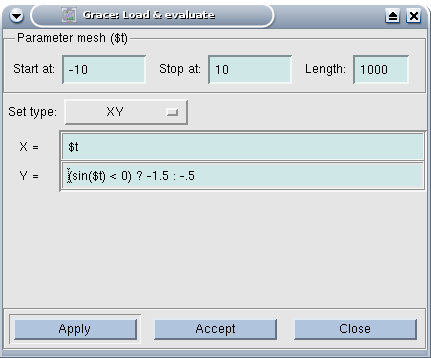
You can also use tests (use of the « ? » characters) equivalent of a « then » and « : » equivalent of an « else ») in the formulas, as in the following examples:
|
|
|
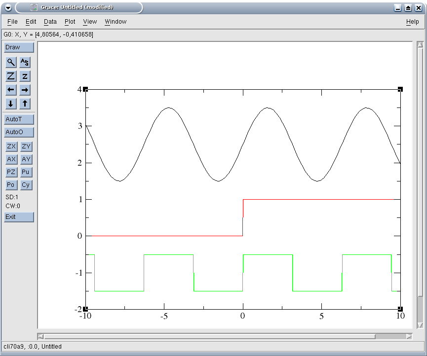
|
You can also use the symbol PI:

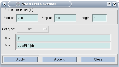
: label: EQ-None
2.3. Duplicating and modifying existing data#
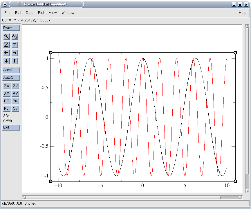
Suppose Grace already has the following curve:
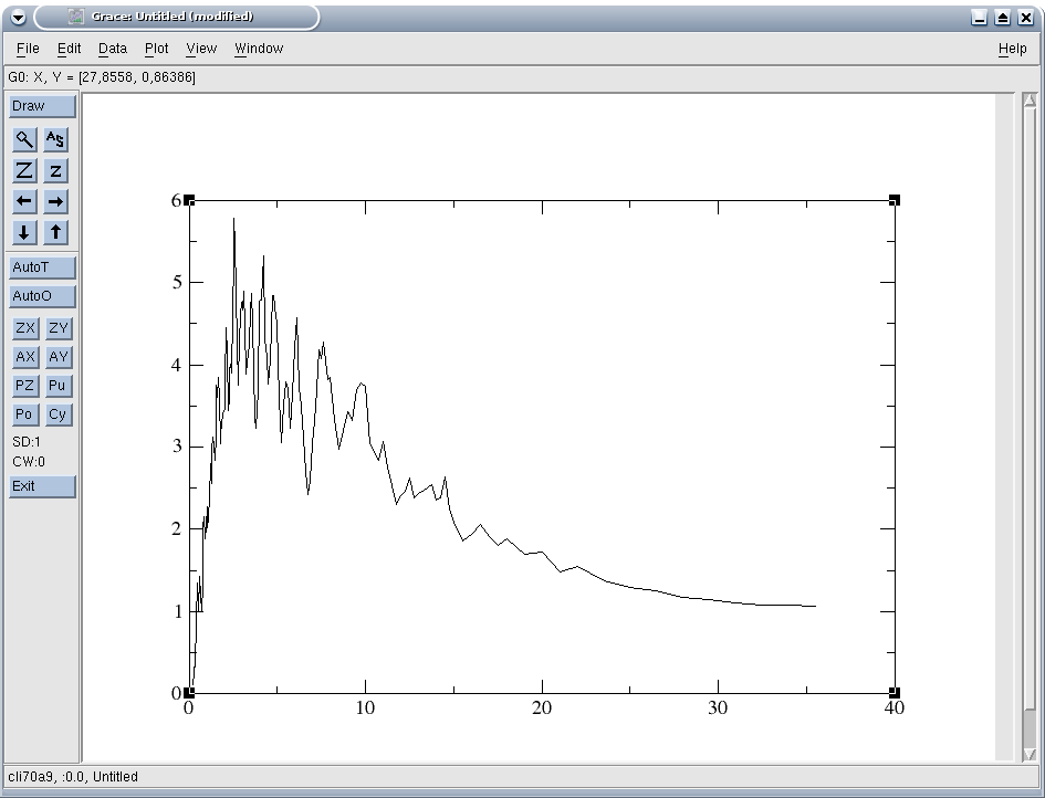
To duplicate/modify a curve, there are two solutions. Whatever the solution chosen, it is necessary to open the control console. With the first solution, you start by duplicating the curve to modify it in the control console; with the second, everything is done in the control console.
2.3.1. Duplication then modification in the console#
It is assumed that there is at least one curve available in Grace.
The command sequence is as follows:
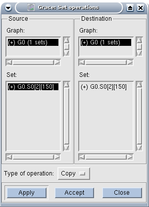
Edit/Set Operations,
select G0 as the graph to copy, S0 as the curve to copy and G0 as the destination graph and « copy » as the operation to be performed, finally « accept »,
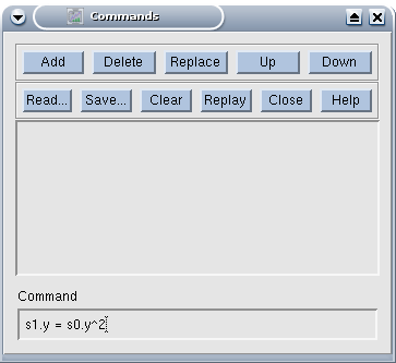
you now have to modify column Y of set S1; this is done by opening the command console: Window/Commands, and typing « s1.y = s0.y^2 » to get the previous curve squared (Cf. [§5.4] from the User’s Guide for a complete list of authorized transactions).
|
|
2.3.2. creation in the console#
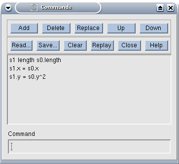
We immediately open the command console: Window/Commands.
We first create the curve by specifying the number of points (identical to the number of points in the S0 set) « s1 length s0.length »,
then we duplicate the abscissa « s1.x = s0.x »,
finally we define the ordinates « s1.y = s0.y^2 »