4. Choice of behavior model

4.1. Introduction

Concrete is a complex material made up of grains of very different scales: centimeters for aggregates, millimeters for sand, tens of microns for cement… Each of these components has different mechanical properties and the interfaces between components cause significant heterogeneities in the material. In addition, the use of concrete during construction is likely to generate non-uniform spatial distributions of components.

Moreover, although these phenomena are not taken into account here, it is important to note that concrete is a multiphase material (presence of water and steam in the interstices) and aging material. Over time, it undergoes phenomena of thermohydration, drying and creep, for example.

The sensitivity of the responses is significant depending on the choice of concrete threshold parameters, as well as post-peak behavior. It is therefore important to adjust the parameters of the law of behavior as best as possible, in particular to calibrate the value of the moment of cracking.

The advantage of carrying out an analysis of the cyclical flexion-membrane response of a reinforced concrete element representative of the section (of the wall, of the slab, etc.) is emphasized before starting the study of the reinforced concrete building in order to verify the good adequacy of the selected parameters.

4.1.1. Experimental observations

Traction

The traction behavior is of a fragile type. A sudden decrease in stress is observed when tensile breaking strength is reached (Figure 4.1.1-a). The order of magnitude of tensile strength is approximately 10 times lower than that of compressive strength. The behavior is almost linear and reversible until breakage. The cracking develops in the direction orthogonal to the load.

For the cyclical behavior under traction, we observe:

• a loss of stiffness during cycles (reduction in the elastic modulus in case of recharging),

• an appearance of irreversible deformations when discharging from a non-linear state.

Compression

The compression behavior of concrete is ductile. The observation of the stress curve - compression deformation (Figure 4.1.1-b) makes it possible to distinguish 3 phases:

• up to stress levels reaching approximately 40% of the maximum stress at the peak (\({\sigma }_{c}\)), the behavior is almost elastic;

• from 40 to 100% of \({\sigma }_{c}\), the behavior gradually becomes non-linear. Near the peak the behavior is highly anelastic. The cracking develops in the direction parallel to the load. A phenomenon of volume expansion (increase in the Poisson’s ratio) is observed. In case of discharge, irreversible deformations appear;

• beyond the peak, the observed behavior becomes softening: the post-peak slope becomes negative.

For the cyclic behavior under compression, we observe:

• a loss of stiffness during cycles (reduction in the elastic modulus in case of recharging);

• an appearance of irreversible deformations when discharging from a non-linear state;

• hysteresis of charge-discharge cycles.

Cyclic

The observation of the stress curve - tensile deformation - cyclic compression (Figure 4.1.1-c) highlights two important aspects:

• the asymmetry of the thresholds in tension and compression (\({\sigma }_{c}=10{\sigma }_{t}\) approximately);

• the closure of cracks. Stiffness is restored in compression when the cracks are closed (unilateral effect).

Figure 4.1.1-a : experimental response of concrete under cyclic traction (from ) .	Figure 4.1.1-b : experimental response of concrete under cyclic compression (from ) .
Figure 4.1.1-c : experimental response of concrete under tension — compression (from ) .

4.1.2. Specificities of seismic studies

In seismic studies, it is first of all imperative to correctly represent concrete cracking under tension:

• sudden decrease in post-peak stress,

• reduction in the discharge module,

• appearance of irreversible deformations.

Given the cyclical aspect of seismic loads, it is then essential to take into account the unilateral aspect of concrete:

• asymmetry of the thresholds,

• closing cracks (regaining stiffness).

Finally, depending on the level of stress achieved in compression in the study, it is necessary to correctly represent the ductile nonlinear behavior of concrete under compression:

• non-linear increase in stress up to the peak then softening,

• reduction in the discharge module,

• appearance of irreversible deformations.

The models capable of representing (more or less accurately) these phenomena are the following:

• ENDO_ISOT_BETON [R7.01.04],

• ENDO_ORTH_BETON [R7.01.09],

• MAZARS_UNIL [R7.01.08],

• GLRC_DM [R7.01.32].

Other concrete models exist in Code_Aster but their use is not recommended. This is the case for example with the models by Mazars [R7.01.08], Double Drücker-Prager [R7.01.03] and BETON_REGLE_PR [U4.43.01] (non-linear elastic and therefore non-dissipative). These models do not allow the reclosing of cracks to be simulated and are therefore not adapted to the case of cyclic loading.

4.2. De Borst algorithm

Before detailing the various models available, we recall that there is in Code_Aster a general method for integrating 3D nonlinear behavior models in plane constraints (Deborst method, [R5.03.03]). This consists in making the \({\sigma }_{\mathrm{zz}}\) constraint in solving the problem null.

The De Borst method has also been generalized to 1D models. A uniaxial stress hypothesis is imposed (\({\sigma }_{\mathit{yy}}\mathrm{=}{\sigma }_{\mathit{zz}}\mathrm{=}0\)). As a result, 3D behavior models can be used for modeling multifibre beams.

The keyword RESI_CPLAN_RELA makes it possible to relax the convergence criterion of the method (verification of the condition of plane constraints). It is recommended for seismic studies to keep RESI_CPLAN_RELAà \({10}^{\mathrm{-}6}\) (value by default). In addition, it is recommended to take a value of RESI_CPLAN_RELA identical to that of the relative residue on the RESI_GLOB_RELA equilibrium. If the convergence criterion is not met, the calculation stops (or there is a redistribution of the time step).

The keyword ITER_CPLAN_MAXI can be used to better satisfy the plane stress condition. By default this parameter is set to 1 (sufficient value for non-softening models). If convergence problems are observed during iterations due to the De Borst algorithm, it is recommended to increase the value of this parameter. For example, we could take “ITER_CPLAN_MAXI” equal 5 or 10. If the convergence criterion is not met after the defined number of iterations, the calculation stops (or there is a redistribution of the time step).

The choice of the value of ITER_CPLAN_MAXI depends on the resolution operator used in Newton’s method (see § 7.2.3):

• if we use the tangent matrix, we can first take the value by default ITER_CPLAN_MAXI =1. In case of non-convergence, it is possible to test a higher value;

• if we use the elastic matrix or the discharge matrix it is recommended to directly take a higher value of ITER_CPLAN_MAXI (we recommend doing between 5 and 10 iterations) otherwise the plane stress condition may not be respected.

4.3. Description of steel behavior models

This section briefly presents the behavior models that can be used to represent the steel material in the context of seismic studies. In Tableau 1, we summarize the different models available depending on the modeling used.

	Modeling BARRE	Multifiber modeling POU_D_EM	Modeling GRILLE_MEMBRANE GRILLE_EXCENTRE
VMIS_ISOT_LINE	X	X
VMIS_CINE_LINE	X	X
PINTO_MENEGOTTO	X	X
GRILLE_ISOT_LINE			X
GRILLE_CINE_LINE			X
GRILLE_PINTO_MEN			X

Table 1 : steel behavior models.

This document does not detail the behavior models of steels. These models are described in [R5.03.09] and [U4.51.11].

Let’s just note that:

• the Von Mises model with symmetric linear isotropic work hardening (VMIS_ISOT_LINE) and the Von Mises model with symmetric linear kinematic work hardening (VMIS_CINE_LINE) are classical elastoplastic models;

• model PINTO_MENEGOTTO makes it possible to represent the uniaxial elastoplastic behavior of reinforced concrete reinforcements. This model reflects the non-linearity of bar work hardening under cyclic loading and takes into account the Bauschinger effect. It also makes it possible to simulate the buckling of reinforcements under compression.

In seismic studies, deformation levels in steels remain relatively low for the most part. The use of a Von Mises elastoplastic behavior model with kinematic work hardening is sufficient. When you want to represent the plastic behavior of steels in a more detailed way, you can use the Pinto - Menegotto model.

4.4. Description of concrete behavior models

In this section, the behavior models that can be used to represent concrete material in the context of seismic studies are presented. In Tableau 2, we summarize the different models available depending on the modeling used.

	Massive 3D	2D Plane Constraints	2D Global	1D Fiber
ENDO_ISOT_BETON	X	X (De Borst)		X (De Borst)
ENDO_ORTH_BETON	X	X (De Borst)		X (De Borst)
MAZARS	X	X	X	X
GLRC_DM	—	–	–	X	–
DHRC	–	–	X	–

Table 2 : concrete behavior models or reinforced concrete.

4.4.1. Model ENDO_ISOT_BETON

This three-dimensional model ([R7.01.04] and Error: Reference source not found]) is based on damage theory (Figure 4.4.1-a and Figure 4.4.1-b), with the damage variable being scalar (isotropic damage). The main advantages of this model are its simplicity (two or three input parameters) and its thermodynamically based theoretical writing.

Determining model parameters:

We have 3 parameters for the model ENDO_ISOT_BETON [U4.43.01] in addition to the classical elastic parameters \(E\) (Young’s modulus) and \(\nu\) (Poisson’s ratio):

• SYT is the maximum stress in simple tension. The value of this parameter is a classical experimental data for concrete. SYT is generally in the range of 1 to 4 MPa (Figure 4.4.1-a);

• D_ SIGM_EPSI is the slope of the post-peak curve under tension (Figure 4.4.1-a). This parameter plays a major role in the response of the structure. It is necessary to use a sufficiently steep post-peak slope so that the spread of damage is correctly represented by the calculation. However, the use of a realistic post-peak slope leads to significant convergence problems. In fact, the more softening the behavior of the material is, the more difficult the convergence becomes. The value of this parameter is approximately -0.2 to -0.6 times Young’s modulus. In practice, it is often necessary to reduce the value of this parameter in order not to have a non-convergence of the calculation;

• SYC is the elastic limit in simple compression. It should be noted that model ENDO_ISOT_BETON is almost linear in compression (no nonlinearity in compression). The use of this optional parameter makes it possible to make the damage threshold dependent on confinement [R7.01.04]. For stresses less than SYC, we have realistic linear concrete behavior. Beyond SYC (elastic limit), the model is no longer representative of the behavior of concrete. SYC is worth about 10 times the stress at peak tension SYT, in absolute value. If this parameter is not used, the elastic compression limit is taken to be in the order of SYT, which is too low. The use of this parameter is therefore recommended, all the more so as it does not seem to worsen convergence problems.

Internal variables:

• \(\mathrm{V1}\): damage value,

• \(\mathrm{V2}\): damage indicator (0 for the elastic regime (zero damage), 1 if damaged, 2 if broken (damage equal to 1)).

ENDO_ISOT_BETON allows you to model:

• the fragile behavior of concrete under tension;

• the unilateral behavior of concrete (closing cracks by regaining stiffness).

ENDO_ISOT_BETON does not allow modeling:

• nonlinear compression behavior;

• the anisotropy of the material;

• irreversible deformations in compression and tension;

• the hysteresis loops in charge - discharge.

Figure 4.4.1-a : relationship \((\sigma -\epsilon )\) in cyclic tract ENDO_ISOT_BETON .	Figure 4.4.1-b : relationship \((\sigma -\epsilon )\) in traction — cyclic compression ENDO_ISOT_BETON .

4.4.2. Model ENDO_ORTH_BETON

This three-dimensional model [R7.01.09] is based on damage theory (Figure 4.4.2-a and Figure 4.4.2-b). It is chosen to introduce two damage variables:

• a \(D\) tensor of order 2 relating to the damage created during traction. This makes it possible to describe the preferred orientation of the cracks orthogonally to the direction of greatest traction (anisotropic damage);

• a scalar d relating to the damage created during compression (isotropic damage).

We have 6 parameters for the model ENDO_ORTH_BETON [U4.43.01] (Tableau 3), in addition to the classical elastic parameters \(E\) (Young’s modulus) and \(\nu\) (Poisson’s ratio).

	Code_Aster	Definition	Dimension
\(\alpha\)	ALPHA	Coupling parameter	without
\({k}_{0}\)	K0	Constant part of the threshold	\(\mathrm{MPa}\)
\({k}_{1}\)	K1	Threshold Parameter	\(\mathrm{MPa}\)
\({k}_{2}\)	K2	Threshold Parameter	Without
\({\gamma }_{B}\)	ECROB	Blocked volume energy relating to traction	\(\mathrm{MPa}\)
\({\gamma }_{d}\)	ECROD	Blocked volume energy related to compression	\(\mathrm{MPa}\)

Table 3 : model parameters ENDO_ORTH_BETON.

Determining model parameters:

• for parameter \(\alpha\), a value between 0.85 and 0.9 is recommended;

• parameters \({k}_{0}\) and \({\gamma }_{B}\) must be identified simultaneously on a simple tensile test;

• the parameters \({\gamma }_{d}\), \({k}_{1}\) and \({k}_{2}\) must be identified simultaneously on a simple compression test.

It is imperative to refer to the documentation [R7.01.09] and to the test cases [V6.04.176] in which the choice of model parameters is discussed in detail.

Internal variables:

• \(\mathrm{V1}\) to \(\mathrm{V6}\): tensile damage tensor;

• \(\mathrm{V7}\): compression damage.

ENDO_ORTH_BETON allows you to model:

• the fragile behavior of concrete under tension;

• nonlinear compression behavior;

• the unilateral behavior of concrete (closing cracks by regaining stiffness);

• the anisotropy of the material.

ENDO_ORTH_BETON does not allow modeling:

• irreversible deformations in compression and tension;

• the hysteresis loops in charge - discharge.

+——————————————————————————————————————-+———————————————————————————————————————+——————————————————————————————————————-++ | | | + .. image:: images/101CFBF00000615C000044BBEDE5E26CA6C80BBB.svg + .. image:: images/101D17720000615C000044BB03C1DB6A589E6A35.svg + | :width: 301 | :width: 301 | + :height: 212 + :height: 212 + | | | + + + | | | +——————————————————————————————————————-+———————————————————————————————————————+——————————————————————————————————————-++ |**Figure** 4.4.2-a **: relationship** :math:`(\sigma -\epsilon )` **in cyclic tract** **ENDO_ORTH_BETON** **.** |**Figure** 4.4.2-b **: relationship** :math:`(\sigma -\epsilon )` **in cyclic compression** **ENDO_ORTH_BETON** **.** || +——————————————————————————————————————-+———————————————————————————————————————+——————————————————————————————————————-++

4.4.3. Model MAZARS

This model is based on damage theory [R7.01.08]. Written in three dimensions, it is available in Code_Aster in 1D, 2D, 3D, AXIS, plane constraints. A variation of this model was developed specifically for civil engineering studies: MAZARS_UNIL. Two variables CRITSIG and CRITEPS correspond to the criteria ELS and ELU classically used in civil engineering.

• For 1D behaviors (multi-fiber beams), a MAZARS_UNIL behavior is associated with each concrete fiber of the beam. It corresponds to the 1D spelling of the unilateral Mazars model (Mu model). The main features of this model are as follows:

◦ use of two variables, one associated with tensile damage and the other with compression damage.

◦ management of the opening of cracks and their reclosing by introducing a restoration of damaged stiffness.

• For behaviors other than 1D, the model corresponds to the one described in [R7.01.08] which cannot account for the closure of cracks in case of alternating loading.

Determining model parameters:

Model parameters should be identified based on the classical material characteristics of concrete. We will refer to [R7.01.08] which gives the elements necessary for setting the parameters.

In practice, the use of the DEFI_MATER_GC command makes it possible to quickly define the material parameters based on the characteristics conventionally obtained during a compression test.

MAZARS_UNIL in 1D **** (Mu model) ****allows you to model: **

• the fragile behavior of concrete under tension;

• nonlinear compression behavior;

• the unilateral behavior of concrete (closing cracks by regaining stiffness);

• the hysteresis loops in charge — discharge.

MAZARS_UNIL in modeling other than 1D:

• the fragile behavior of concrete under tension;

• nonlinear compression behavior;

• the unilateral behavior of concrete (closing cracks by regaining stiffness);

• the hysteresis loops in charge — discharge.

4.4.4. Damage-related location and non-local models

Local damage behavior patterns ENDO_ISOT_BETON and ENDO_ORTH_BETON or MAZARS can lead to the localization of deformations. In this case, a concentration of the damage is observed in a band of one mesh thickness. In addition, the energy dissipated by the damage becomes zero when the width of this band tends to 0. The localization phenomenon involves a dependence on the response of the structure to the mesh.

In order to be fixed on the presence or absence of a location, it is therefore advisable, if significant concentrations of damage are observed, to resume the calculation by re-meshing the suspected area more finely. If we note that the damage is always concentrated on the first band of elements (reduction of the damaged area), there is definitely a problem of location.

Moreover, methods for delocalizing behavioral models make it possible to avoid these problems of dependence of the solution on the mesh. In Code_Aster, there is a relocation method available for models ENDO_ISOT_BETON and ENDO_ORTH_BETON: the GRAD_VARI ([R5.04.01]) modeling.

This non-local modeling is currently not available in Code_Aster in nonlinear dynamics (DYNA_NON_LINE) because the inertia operator is not calculated. Moreover, it is also not available for multi-layer shells (only for 3D models or D_ PLAN).

4.4.5. Model GLRC_DM

Model GLRC_DM [R7.01.32] is a « global » reinforced concrete model based on a heuristic homogenization formulation for reinforced concrete plates and shells. It is a damage model formulated in terms of generalized deformation/stress relationships (membrane extension, curvature, distortion and membrane forces, bending moments, shear forces). It has 2 coupled damage variables describing damage by flexion-extension (one for each face of the plate), and therefore the anisotropy induced by the damage. It can be used in thermomechanical situations (fine temperature distribution in the thickness of the reinforced concrete section).

Since the behavior of concrete and steel is homogenized, the overall model is not a softening step. As a result, most non-convergence problems are avoided. In addition, problems in locating the damage are thus avoided. Refer to [R7.01.32] for a detailed description of the model.

The model parameters are as follows [U4.43.01]:

Elastic parameters:

	Definition	Dimension
E	Young’s modulus equivalent in traction (homogenized)	\(\mathrm{Pa}\)
NU	Poisson’s ratio equivalent in traction (homogenized)	without
EF	Young’s modulus equivalent in flexure (homogenized)	\(\mathrm{Pa}\)
NUF	Poisson’s ratio equivalent in flexure (homogenized)	without

Nonlinear parameters

	Definition	Dimension
NYT	(Stress * thickness) corresponding to the damage threshold in pure traction of the homogenized material (1)	\(N/m\)
MYF	Pure flexural damage threshold of homogenized material	\(N\)
NYC	(Stress * thickness) corresponding to the damage threshold in pure compression of the homogenized material	\(N/m\)
GAMMA_T	Parameter managing the damaging (post-elastic) slope defined in relation to the elastic slope under pure traction	without
GAMMA_F	Parameter managing the damaging (post-elastic) slope defined in relation to the elastic slope in pure bending	without
GAMMA_C	Parameter managing the damaging (post-elastic) slope defined in relation to the elastic slope in pure compression	without
ALPHA_C	Parameter for delay in onset of compression damage	without

(1): SYT is defined by: \(\text{SYT}={\sigma }_{\text{élas}}\times h\), with \({\sigma }_{\text{élas}}\) the pure tensile elastic stress limit and \(h\) the thickness of the reinforced concrete shell.

Unlike local models ENDO_ISOT_BETON and ENDO_ORTH_BETON, the post-elastic slopes of model GLRC_DM (\({P}_{p\mathrm{trac.}}\) and \({P}_{p\mathrm{flex}}\)) are positive because they represent the overall behavior of damaged concrete and elastoplastic steels.

Determining model parameters:

The four main parameters to be identified are:

• the elastic threshold SYT and the post-elastic membrane slope GAMMA_T;

• the elastic threshold SYF and the post-elastic flexural slope GAMMA_F.

In order to fine-tune the model, it is also possible to take a DeYoung’s modulus and a Poisson’s ratio in flexure (EF and NUF) different from those taken in a membrane. In fact, as reinforced concrete is not a homogeneous material, the effective value of EF may be different from E (apparent flexural stiffness). Therefore, the user is left with the possibility of entering a value of EF (under the keyword GLRC_DM) independent of E.

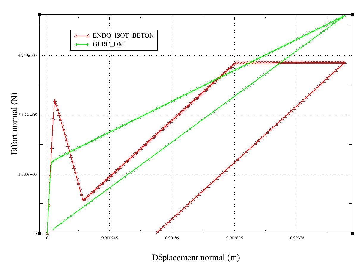
For identification, two methodologies exist. The first identification methodology consists in adjusting the parameters GLRC_DM with respect to the model DKT - ENDO_ISOT_BETON (concrete) + GRILLE - VMIS_CINE_LINE (reinforcements) on an elementary tension-compression test, then on an elementary flexure test.

Traction — compression:

It is advisable to use test case SSNS106A [V6.05.106] which treats the case of cyclic traction-compression to identify the parameters SYT and GAMMA_T. We get a response curve shown Figure 4.4.5-a.

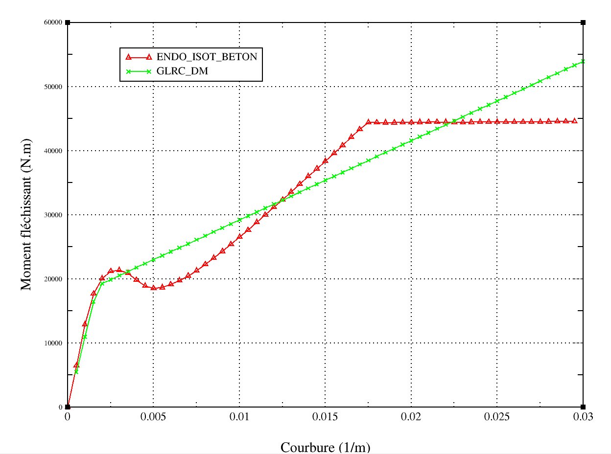
Flexion:

It is advisable to use test case SSNS106B [V6.05.106] which treats the case of cyclic flexure to identify the parameters SYF and GAMMA_F. In addition, it is possible to adjust the parameters EF and NUF (elastic parameters of the reinforced concrete plate under bending). We get a response curve shown Figure 4.4.5-b.

In order to adjust the parameters of model GLRC_DM, the user may wish to maintain the overall approach compared to a more realistic model:

• the initial elastic stiffness (and therefore the initial natural frequency),

• the elastic limit,

• energy dissipation (or damping) defined by the area of the response curve over a cycle,

• the maximum deformation reached,

• the deterioration of stiffness.

On Figure 4.4.5-a and Figure 4.4.5-b, the adjustment was carried out in such a way as to have approximately the area under the two curves (ENDO_ISOT_BETON and GLRC_DM) identical in the load range \((\epsilon -\sigma )\) referred to in the seismic analysis (equivalent to the energy dissipated). In addition, an attempt was made to keep elastic limits close in both models.

Figure 4.4.5-a : answer GLRC_DM and ENDO_ISOT_BETON - traction-compression test.	Figure 4.4.5-b : answer GLRC_DM **** and**** ENDO_ISOT_BETON ****- flexure test. **

This methodology is the most accurate. However, it poses implementation time problems. Indeed, it quickly becomes tedious to carry out this adjustment when it is necessary to study dozens of sails and floors. To overcome this difficulty, the command DEFI_GLRC [U4.42.06], initially developed to automatically determine the parameters of the law of behavior GLRC_DAMAGE, has been enriched. It allows the identification of the parameters of GLRC_DM based on the knowledge of the geometric and material data of the various components of the reinforced concrete slab.

Internal variables:

• \(\mathrm{V1}\): damage on the upper side,

• \(\mathrm{V2}\): damage to the side of the underside,

• \(\mathrm{V3}\): damage evolution indicator \(\mathrm{V1}\). \(\mathrm{V3}\) is 1, when \(\mathrm{V1}\) evolves and 0 otherwise,

• \(\mathrm{V4}\): damage evolution indicator \(\mathrm{V2}\). \(V4\) is 1, when \(V2\) evolves and 0 otherwise.

• \(V5\): relative weakening of stiffness under tension

• \(V6\): relative weakening of stiffness under compression

• \(V7\): relative weakening of stiffness during bending

In addition, the « internal variables » \(V8\), \(V9\),, \(V10\) and \(V11\) are introduced in order to facilitate post-treatments on steel reinforcements. These variables depend on limit deformations EPSI_ELS (limit to ELS) and EPSI_LIM (limit to ELU), which are provided via DEFI_MATERIAU/GLRC_DM. See [R7.01.32].

The « internal variables » \(V12\), \(V13\), \(V14\), \(V15\) and \(V16\) are also introduced in order to easily access the extreme temporal tensile and compressive deformations in concrete, on the upper face and on the lower face. See [R7.01.32].

Finally, the « internal variables » \(V17\) and \(V18\) are introduced in order to assess the validity of the parameters that have been chosen.

4.4.6. Model GLRC_DM coupled with elastoplasticity (VMIS_CINE_LINE)

In order to take into account the elastoplastic phenomenology of behavior and thus better represent the hysteresis of the cyclic response of a reinforced concrete structure, Code_Aster has a numerical platform for coupling damaging and elastoplastic models [22]. Model GLRC_DM is coupled with a Von Mises model (VMIS_CINE_LINE) for the membrane part only (it is completed by an elastic flexural model) [R7.01.19].

To summarize, the GLRC_DM + VMIS_CINE_LINE behavior model makes it possible to represent membrane-flexural damage and membrane plasticity.

It is recommended to proceed step by step in the use of model GLRC_DM coupled with membrane elastoplasticity: we will first perform a calculation with the simple GLRC_DM model and then we will implement this more complex model.

In operator DYNA_NON_LINE, the RELATION_KIT operand is used. The keyword associated with concrete behavior combinations is” KIT_DDI “. This keyword makes it possible to add the two anelastic deformation terms defined by the laws of behavior GLRC_DM and VMIS_CINE_LINE existing in COMPORTEMENT:

COMPORTEMENT = _F (RELATION = 'KIT_DDI'

RELATION_KIT = ('GLRC_DM', 'VMIS_CINE_LINE'))

The required material field data must be provided in operator DEFI_MATERIAU. Refer to test case SSNS106 [V6.05.106] for more details on the syntax.

Determining model parameters

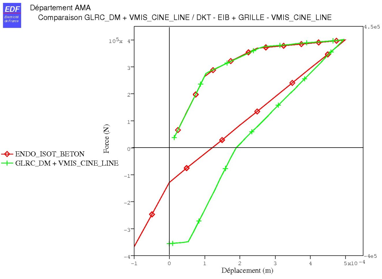
The methodology currently implemented consists in identifying the parameters GLRC_DM + VMIS_CINE_LINE in membrane compared to the model DKT - ENDO_ISOT_BETON (concrete) + GRILLE - VMIS_CINE_LINE (reinforcements) on an elementary tensile — compression test.

It is recommended to use test case SSNS106F which treats the case of cyclic traction-compression for the GLRC_DM + VMIS_CINE_LINE model. We get a response curve shown Figure 4.4.6-a.

Figure 4.4.6-a : elementary response — traction-compression test.

Internal variables

The internal variables of each law are accumulated in the table of internal variables, and restored law by law (4 internal variables for GLRC_DM then 7 internal variables for VMIS_CINE_LINE).

4.4.7. Model DHRC

Model DHRC [R7.01.37] is a « global » reinforced concrete model based on a formulation by numerical homogenization, first using resolutions at the scale of a V.E.R., representative of the reinforced concrete section, with dimensions equal to the transverse reinforcement steps, for reinforced concrete plates and shells.

The specific goals of the DHRCsont model:

• flexion-membrane coupling and representation of any sections, based on the distribution of steels in the V.E.R.;

• modeling of damage and stiffness reduction, associated dissipation;

• modeling of steel-concrete sliding and irreversible deformations, tension, stiffening and associated dissipation.

Figure 4.4.7-a: see for model DHRC.

Internal variables:

• \(\mathrm{V1}\): damage on the upper side,

• \(\mathrm{V2}\): damage to the side of the underside,

• \(\mathrm{V3}\): steel-concrete sliding according to \(x\) upper reinforcement bed,

• \(\mathrm{V4}\): steel-concrete sliding according to \(y\) upper reinforcement bed,

• \(\mathrm{V5}\): steel-concrete sliding according to \(x\) lower reinforcement bed,

• \(\mathrm{V6}\): steel-concrete sliding according to \(y\) lower reinforcement bed,

• \(\mathrm{V7}\): density of energy dissipated by damage (accumulation),

• \(V8\): density of energy dissipated by steel-concrete sliding (cumulation),

• \(V9\): total dissipated energy density (cumulative),

• \(V10\): relative weakening of membrane stiffness due to damage,

• \(V11\): relative weakening of flexural stiffness due to damage.

4.5. What type of behavior model should you adopt?

4.5.1. Introduction

The choice of the behavior model is closely linked to the modeling adopted. In Tableau 4, we summarize the various possible modeling strategies.

In order to choose the model of behavior adapted to our problem, it is necessary to answer the following questions:

• What is the maximum stress level that we want to apply to the structure (damage level) and what is the robustness of the concrete behavior model?

• low damage: few risks of non-convergence;

• high damage: risks of non-convergence becoming high;

• what mechanical phenomena do we want to represent?

• damage to concrete (tensile/compression);

• damage to concrete and plasticity of steels and concrete.

The advantages and disadvantages associated with each type of behaviour model are presented below. These questions are answered for each type of model.

4.5.2. Model ENDO_ISOT_BETON

Advantages:

• it is a simple 3D concrete behavior model,

• the identification of the parameters is immediate.

Disadvantages:

• we represent the damage to concrete under tension only,

• there are significant non-convergence problems when the damage becomes high.

Note

The model ENDO_ISOT_BETON used in plane constraints via the Deborst method for multi-layer shells is in principle more robust than its three-dimensional version. In practice, however, convergence problems are observed when the damage becomes too high in the structure.

4.5.3. Model ENDO_ORTH_BETON

Advantages:

• it is a 3D model allowing to finely represent the damage of concrete in tension and compression.

Disadvantages:

• there are significant problems of non-convergence when the damage becomes high,

• the determination of the parameters requires a relatively complex preliminary calibration.

Note

The model ENDO_ORTH_BETON used in plane constraints via the Deborst method for multi-layer shells is in principle more robust than its three-dimensional version. In practice, however, convergence problems are observed when the damage becomes too high in the structure.

4.5.4. Model MAZARS_UNIL [R7.01.08]

Advantages:

• In 1D (used with multifibre beams [R5.03.09]):

◦ as the model is written in 1D, non-convergence problems are significantly reduced;

◦ it makes it possible to finely represent mechanical phenomena in the longitudinal direction (traction — compression and bending); the model is capable of accounting for the phenomenon of reclosing cracks.

• In 2D, 3D, C_ PLAN:

◦ makes it possible to represent shear phenomena, and makes it possible to translate the phenomenon of crack closure (restoration of stiffness).

4.5.5. Model GLRC_DM [R7.01.32]

Number of parameters: steel: 3, concrete: 8, geometry: 5, method: 2. But these parameters are provided in Code_Aster based on « engineer » data and hypotheses about the post-elastic deformation range.

Advantages:

• the softening behavior of concrete is no longer modelled. As a result, most non-convergence problems are avoided;

• in the same way, as we homogenize the behavior of concrete and steel, we avoid location problems;

• the GLRC_DM + plasticity model makes it possible to model residual deformations (in membrane only).

Disadvantages:

• the identification of the parameters requires a readjustment work compared to a more precise model such as ENDO_ISOT_BETON.

• Steel reinforcement sheets necessarily identical x-y, sup-inf.

• step no flexion-membrane coupling

4.5.6. Model DHRC [R7.01.37]

Number of parameters: steel: 3, concrete: 10, steel-concrete slip: 1, geometry: 11.

Advantages:

• Plates of steel reinforcements of any kind,

• Native anisotropy,

• Steel-concrete slip resulting from damage and therefore contribution to the dissipation and modeling of the « tension-stiffening effect » phenomenon,

• native flexion-membrane coupling

• Automated identification tool by EF numerical homogenization of parameters in Salomé_Méca based on « engineer » data.

Disadvantages:

• CPU: more expensive than GLRC_DM: 30 to 100%,

• ways of progress are expected on tests to characterize the steel-concrete bond: at this stage of the state of the art, this restriction weakens the predictive capacity of this modeling;

• Industrialization and validation on representative structures (experimental campaigns) to be completed.

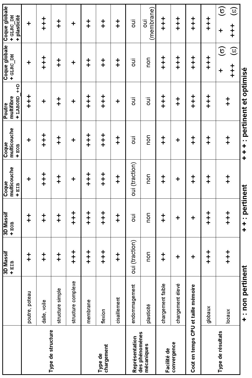
Table 4 : summary of the choice of modeling and the associated behavior model.