3. Choice of finite element modeling#
3.1. Introduction#
The aim is to represent two main families of reinforced concrete structural elements present in conventional civil engineering buildings:
beams and columns,
radiators, floors (slabs) and walls.
There are three main categories of finite element representations:
Local representation (massive elements)
In this classical finite element approach, the constituent materials (steel and concrete) are modelled separately. Massive finite elements are used for concrete and the associated behavior models are written in 3D. The discrete modeling of steels with finite element bars creates stress singularities, which is very disadvantageous as soon as. That we switch to a non-linear regime of behavior, cf. [21]. This type of approach makes it possible to obtain a detailed description of the nonlinear phenomena involved but its application to the entire industrial type of structure can be difficult (time CPU and memory size are prohibitive). In addition, the use of local behavioral models leads to penalizing non-convergence problems.
Semi-global representation
The models used are multi-layer beams and shells and integration is carried out in the thickness of the element. The constituent materials are always modelled separately. We can distinguish between:
multi-layer shells supported by shell-type finite elements. Simplifying hypotheses associated with shell theory are adopted (the displacement fields vary linearly in the thickness of the shell, the transverse stress \({\sigma }_{\mathrm{zz}}\) is zero). The associated behavior models are written in 2D plane constraints;
multifibre beams supported by finite beam-type elements. Simplifying hypotheses associated with the theory of Euler beams are adopted (the sections remain straight and perpendicular to the average fiber). The associated behavior models are written in 1D for concrete fibers and steel fibers.
The main advantage of this type of modeling is to be much less expensive in terms of time CPU and in memory size than a traditional local representation. It also makes it possible to represent the structure to be studied in a relatively realistic manner. Post-treatments are available to access quantities of interest to engineers.
Global representation
In this approach, the overall behavior of reinforced concrete is modelled (the constituent elements are no longer considered separately). Finite support elements are single-layer structural elements (beams, shells). The associated specific behavior patterns are written in global variables (generalized efforts, generalized deformations). Global models are generally developed for specific applications (for a type of component of a structure, for a type of stress,…). This type of representation is very inexpensive in terms of time CPU and memory size, but modeling data requires identification that must be done carefully. Moreover, this identification is generally only valid for one load class.
The following Figure 3.1-a illustrates the types of models available in*Code_Aster*.
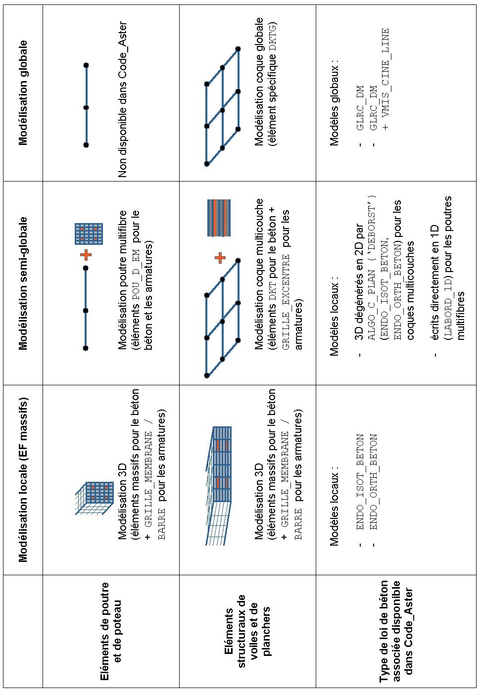
Figure 3.1-a : summary of the types of models available.
3.2. Description of local modeling (massive elements)#
3.2.1. Concrete modeling#
Modeling using classical solid finite elements is not covered in this document since it does not have its own specific characteristics in the case of concrete, cf. also u2.03.07. Refer to the general documentation of*Code_Aster* for any modeling problems.
3.2.2. Reinforcement modeling#
The following two types of modeling can be used to represent reinforcement reinforcements:
bar elements (BARRE, [U3.11.01]). These linear finite elements in 3D space only transmit axial forces and deformations. On the other hand, in dynamics, inertia forces appear in all directions. The use of elements BARREimplique to model all the reinforcements one by one. This modeling is to be used when the reinforcement is complicated and when one seeks to represent the geometric position of the reinforcements in a very fine way; however, we will take care of the difficulties reported in [21];
membrane grid elements (GRILLE_MEMBRANE, [U3.12.04]). This modeling GRILLE_MEMBRANE makes it possible to represent reinforcement sheets with a single reinforcement direction working as a membrane only. Finite support elements are surface elements (TRIA3, QUA4,…). The concept of eccentricity does not exist for this modeling. It is therefore necessary to position the reinforcements in the right place when meshing the structure. To represent a complete frame bed (reinforcement in two orthogonal directions), the first GRILLE_MEMBRANE bed is duplicated and a second bed orthogonal to the first is defined.
Note
It has been shown that the mixture of massive elements (concrete) and bar (steel) can introduce singularities that are a source of non-convergence in relation to the mesh size and in the resolution of the nonlinear balance * (application of a point load) [21] . It is therefore preferable, if the problem allows it, to use the grid elements to represent the reinforcements.
3.2.3. Modeling the connection between concrete and reinforcements#
It is recommended to make the nodes of the steel and concrete meshes coincide to ensure the continuity of movements at the interface. This makes it possible not to increase the size of the problem because it is thus avoided to introduce bond relationships between the steel and concrete meshes in order to ensure adherence. It is necessary to properly match all the concrete nodes located along the reinforcement with a steel node.
The reinforced concrete structure is then represented by the superposition of the BARREou GRILLE_MEMBRANE elements used for steels and the massive 3D elements used for concrete.
It should be noted that this modeling strategy implies that the steel-concrete bond is perfect. This is reductive of the true phenomenology of the behavior of reinforced concrete sections for which steel-concrete sliding (delayed by the use of notched or high-adhesion reinforcements) produces the transition to a regime described by the « tension stiffening effect » for which we obtain a response of the section much more resistant than that predicted by the sole contribution of the steels once the concrete has cracked.
More realistic models of the bond between steels and concrete are available in Code_Aster:
In 2D: JOINT_BA, [R7.01.21]. It is not suitable for seismic applications on a complete building. It can be used to study a steel-concrete bond locally (pull-out test, for example).
In 3D: cohesive law CZM_LAB_MIX, [R7.02.11], [7]. It makes it possible to model the sliding of steel reinforcements in relation to concrete. The sliding surface is discretized by finite interface elements, see [R7.02.13].
3.3. Description of multi-layer shell semi-global modeling#
3.3.1. Concrete modeling#
Concrete is modelled using Code_Aster plate or shell elements (DKT, DST, Q4G, COQUE_3D, COQUE_SOLIDE). This document does not go back to the formulation of these elements. Refer to [U2.02.01] for their use.
We simply recall that since the calculations carried out are non-linear, we use a method of integration by layer for these elements. For each layer, a Simpson method is used with three integration points, in the middle of the layer and in upper and lower layers. For \(N\) layers the number of integration points in the thickness is \(2N+1\). For tangent stiffness, for each layer, under plane stresses, the contribution to the membrane stiffness, and membrane-flexure coupling matrices as well as the contribution to generalized internal forces are calculated. These contributions are added and assembled to obtain the total tangent stiffness matrix.
To treat material nonlinearities, it is recommended to use 3 to 5 layers in the thickness for a number of integration points equal to 7, 9 and 11 respectively.
3.3.2. Reinforcement modeling#
The following two types of modeling can be used to represent reinforcement reinforcements:
bar elements (BARRE, cf. § 3.2.2);
grid items (GRILLE_EXCENTRE, [:external:ref:`U3.12.04 <U3.12.04>`]). This modeling GRILLE_EXCENTRE makes it possible to represent reinforcement sheets with a single reinforcement direction with eccentricity. The position of the reinforcement bed in relation to the mean plane of the reinforced concrete shell is thus defined. To represent a complete frame bed (reinforcement in two orthogonal directions), the first GRILLE_EXCENTRE bed is duplicated and a second bed orthogonal to the first is defined. You only mesh a shell that you duplicate in*Code_Aster in order to create the mesh groups corresponding to the reinforcements (operator CREA_MAILLAGE). All mesh groups rely on the same nodes.
Note
In this semi-global representation of a multilayer shell, it is not possible to model the transverse reinforcements.
3.3.3. Modeling the connection between concrete and reinforcements#
As in § 3.2.3, it is recommended to make the nodes of the steel and concrete meshes coincide and thus ensure the continuity of movements at the interface. This makes it possible not to increase the size of the problem because it is thus avoided to introduce bond relationships between the steel and concrete meshes in order to ensure adherence. If GRILLE_EXCENTRE elements are used for the reinforcements, the steel and concrete nodes naturally coincide because the meshes are duplicated and in fact rely on the same nodes.
The reinforced concrete structure is represented by the superposition of the GRILLE_EXCENTRE models used for the reinforcements and the shell used for the concrete.
3.4. Description of the semi-global multifiber beam modeling#
Multifiber beam modeling (element POU_D_EM, [U3.11.07] and [R3.08.08]) is based on the resolution of a beam problem whose heterogeneous section is divided into several fibers. Each fiber has a uniaxial behavior corresponding to the material from which it is made, while the kinematics is defined by the extension resulting from the specific extension (axial deformation) and from the variation in curvature of the beam itself. The section may be of any shape and is described using a 2D mesh.

|
Figure 3.4-a : multifiber beam modeling of a reinforced concrete beam. |
Remarks
In this semi-global representation of a multifiber beam, it is not possible to model the transverse reinforcements.
The behavior of a reinforced concrete beam is defined by the material data of the concrete fibers and the material data of the steel reinforcing fibers.
The steel-concrete connection is assumed to be perfect: continuity of movements at the interface.
3.5. Global modeling description#
3.5.1. Generalities#
In this type of representation, the structural elements used have only one fiber or layer in the section. The associated homogenized behavior models are written in global variables (generalized efforts, generalized deformations) without using local laws. Most of the developments existing in the literature concern beams. In Code_Aster, however, this type of global reinforced concrete beam elements is not developed.
It should be noted that these global models are very specific (to a type of component element of a structure, to a type of stress,…) and make it difficult to represent in a sufficiently detailed manner the behavior of complex industrial structures. In addition, modeling data requires identification that must be carried out carefully.
3.5.2. Reinforced concrete plate modeling#
The reinforced concrete plate modeling available in Code_Aster is similar to the one that was initially developed in the Europlexus [8] calculation code in order to deal with rapid dynamic problems for civil engineering structures.
The support elements are DKTdégénérés with a single point of integration into the thickness (elements DKTG). This modeling (Figure 3.5.2-a) uses global variables (\(N\), membrane forces; \(M\), flexure moments;, \(\epsilon\) generalized deformations and \(\kappa\), curvatures) from a global behavior model (for reinforced concrete, model GLRC_DM). This model makes it possible to simulate the behavior of reinforced concrete plates under cyclic loading.
Behavior model GLRC_DM is described in more detail in paragraph § 4.4.5 and behavior model DHRC in paragraph § 4.4.7.

|
Figure 3.5.2-a: model of an overall reinforced concrete plate. |
3.6. Link modeling#
It is possible to connect different models to each other depending on the areas of the structure. The various possible modeling approaches are not described here in detail. However, some modeling points are specified.
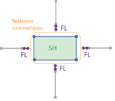
3.6.1. Hull — shell connection#
The connection between two perpendicular shells can be made directly even if, from a greater point of view, the transmission of torsional forces is not exact (the degree of freedom of rotation generating the twist is not transmitted).
If you want to represent the connection between two perpendicular shells in a more precise way, it is possible to do so using linear relationships (in order not to count twice the volume at the intersection of the two shells). To do this, you must use the AFFE_CHAR_MECA, LIAISON_COQUE, [U4.44.01], and [U2.02.01] operators.
The multi-layer shell-global shell connection is natural because the finite elements concerned have the same degrees of freedom.
3.6.2. 3D connection — beam and shell — beam#
In Code_Aster there is an operator that allows you to connect a massive part to a beam (AFFE_CHAR_MECA, LIAISON_ELEM, OPTION =”3D_ POU “, [R3.03.03] and [U4.44.01]), or a shell to a beam (AFFE_CHAR_MECA, LIAISON_ELEM,, OPTION =” COQ_POU”, [ R3.03.06], [U4.44.01], and [U2.02.01]).
These links (3D_ POU and COQ_POU) make it possible to connect two parts of extending meshes. It is not intended to model, for example, a connection between a shell and a beam that is connected perpendicularly. We can therefore see that the pole - floor connections cannot be modelled in this way.
In the case of a column-floor connection, if one seeks to transmit torsional forces correctly, it is recommended to make the connection using shells only (see § 3.6.1, above) and possibly to extend the column with beams using a shell-beam connection (Figure3.6.2-a).
Another possibility, used statically, consists in adding fictional beams in the plane of the shell to transmit the forces coming from the column. This solution should be used with care in dynamics because very low masses must be imposed on fictional beams. If the nodes of these beams are not attached to the shell, there is a risk of disturbing the solution (poorly conditioned mass matrix).

|
Figure 3.6.2-a : pole - floor connection. |
If the torsional forces are not preponderant, the beam and the shell can be connected directly (common node). However, with a non-linear behavior of the floor, this can cause a strong dependence on the mesh or even difficulties of convergence due to local force concentrations.
3.6.3. Pole - floor connection#
It is recommended to use the “PLAQ_POUT_ORTH” option from the LIAISON_ELEM keyword of the AFFE_CHAR_MECA, [U4.44.01] operator. In advance, the definition of the trace of the beam section in the floor mesh must be defined with a named group of elements. It is recommended to place the end node of the column at the geometric center of gravity of the path of the beam section in the floor. You can consult test case SDLX301 [V2.05.301]: floor-column building.
In fact, proceeding in this way makes it possible to best respect the validity hypotheses of both the theory of beams and that of plates. Plate theory does not allow the application of a punctual force (this creates a singularity that is certainly manageable in terms of elasticity but creates difficulties in non-linear terms).
3.6.4. 3D connection — shell#
It is generally recommended to fictitiously extend the shell into the 3D mass in order to ensure the kinematic conditions between the two parts.

|
Figure 3.6.4-a : 3D connection — shell. |
3.6.5. Connections or junctions between structural elements: wall and floor (plates)#
We will consult the documentation for using junctions between structural elements [U2.03.10]. This methodology uses, cf. [16], [17]:
the implementation of kinematic links;
a model of non-linear behavior of a flexural junction between a wall and a floor or a raft, made of reinforced concrete, and affected on a discrete element (ball joints), of type DIS_TR on SEG2 meshes, at two nodes, with two nodes, accessible by the keyword JONC_ENDO_PLAS, see §13 [R5.03.17].
|


|
Figure 3.6.5-a: junction between structural elements: wall and floor.
Modeling of non-linear connections (frame nodes; damping device, etc.) using discrete elements ~~~~~~~~~~~~~~~~~~~~~~~~~~~~~~~~~~~~~~~~~~~~~~~~~~~~~~~~~~~~~~~~~~~~~~~~~~~~~~~~~~~~~~~~~~~~~~~~~~~~~~~~~~~~~~~~~~~~~~~~~~~~~~~~~~~~~~~~~~~~~~~~~~~~~~~~~~~~~~~~~~~~~~~~~~~~~~~~~~~~~~~~~~~~~~~ ~~~~~~~~~~~~~~~~~~~
We will consult the documentation for using discrete elements [U2.02.03].
We can represent the behavior of a post-beam, column-floor or other connection by discrete elements DIS_T (translation) and DIS_TR (translation and rotation) [U3.11.02] and models of linear behavior (linear characteristics given in the operator AFFE_CARA_ELEM [U4.42.01]) or of non-linear behavior (material parameters defined with the operator DEFI_MATERIAU []) or non-linear behavior (material parameters defined with the operator []) or non-linear behavior models (material parameters defined with the operator []). U4.43.01], and called via the RELATION operand in the COMPORTEMENT operator [U4.51.11]).
To ensure anti-seismic protection, it is proposed to install shock-absorbing devices within the Civil Engineering structure or between two buildings. These devices are designed to exert unidirectional forces on connections that can be considered as punctual. However, as their anchoring is generally distributed, it will be possible to take advantage of the various structural links presented in the paragraphs above. We will choose discrete elements with two nodes in translation DIS_T. For example, you could use:
DIS_ECRO_CINE [R5.03.17]: allows you to model globally (elastic limit, non-linear work hardening, ultimate load) the non-linear behavior of frame nodes in reinforced concrete or steel gantries (beam-column connection, girder-beam, beam-floor, or even veil-floor on all the intersection nodes between the mesh plates of the wall and the floor…), but assuming a total decoupling between the meshes of the plates of the wall and the floor…), but assuming a total decoupling between the meshes points along the edge line. We can consult test case SSND102 [V6.08.102].
DIS_VISC [R5.03.17]: allows you to model unidirectional shock absorbers with nonlinear generalized Zener type behavior, with power law. We can consult test case SSND101 [V6.08.101].
These models can be used in a static or dynamic transitory analysis on a « physical » basis.
It is also possible to refer directly to a special behavior law assigned to a pair of linked nodes (localized nonlinearities), within a transient dynamic analysis on a modal basis (operators DYNA_TRAN_MODAL [U4.53.21] and DYNA_VIBRA [] and [U4.53.03]). For example, you could use:
DIS_VISC [R5.03.17]: unidirectional shock absorbers with nonlinear generalized Zener type behavior, with power law. We can consult test case SDND107 [V5.01.107].
ANTI_SISM [U4.53.21]: unidirectional shock absorbers with coupled non-linear displacement-speed behavior. This law results from a formulation from the reference [bib22]; we can consult the test case SDND120 [V5.01.120].
3.7. Other structural elements that can be modelled#
3.7.1. Liner modeling#
The liner is a metal shell placed in the inner skin of the enclosure guaranteeing watertightness in the event of an accidental leak. In order to model it, there are two possibilities:
when the concrete is modelled by massive elements (local 3D representation), the liner is modelled directly by a shell at the real position,
when the concrete is modelled by shells (multilayer or global), the liner is modeled by a shell that is eccentric with respect to the average sheet of the concrete shell.
3.7.2. Prestress modeling#
The prestressed steel cables are put under tension in order to compress the concrete of the civil engineering structure. The methodology for implementing prestress in Code_Aster is not presented here. Refer to [U2.03.06] which describes in detail the carrying out of a study with prestressed cables. It should simply be noted that we can use DEFI_CABLE_BP [U4.42.04] with either a massive 3D modeling or a shell modeling of the type DKT or DKTG (GLRC). In addition, it is not necessary to make the cable nodes coincide with the concrete nodes. In fact, the DEFI_CABLE_BP command also makes it possible to create kinematic links that will link the cable nodes with the concrete nodes of the surrounding mesh. On the other hand, this generates a large number of Lagrange multipliers that will make the calculation more complicated. There is therefore a compromise to be found between the ease of carrying out the meshing and the cost of the calculation. The introduction of too many kinematic relationships can become a problem for a transitory seismic study that is already time-consuming.
3.8. What type of modeling should be adopted?#
3.8.1. Introduction#
The choice of finite element modeling is closely linked to the behavior models associated with it. It is therefore necessary to study the models that can be used (concrete in particular) for seismic studies before answering this question entirely. In the following chapter 4, we describe the steel and concrete models available in Code_Aster and we summarize (Tableau 4) the various possible modeling strategies.
In order to choose a model adapted to a given problem, it is necessary to answer the following questions:
what type of structure are we looking to model?
beam, pole/slab, sail,
simple/complex geometry,
What is the size of the problem?
What type of loading is required?
membrane (traction/compression),
bending,
shearing,
what types of results are we looking to analyze?
global quantities (movements, support forces, floor spectra,…),
local quantities (stresses in concrete, deformations in steels,…).
The advantages and disadvantages associated with each type of modeling are presented below. These questions are answered for each type of modeling.
Note
It is possible to connect different models to each other depending on the areas of the structure (multi-layer shells, global shells, multifibre beams,…) .
3.8.2. Local modeling (massive elements)#
Advantages:
it makes it possible to finely represent complex geometries such as frame nodes or areas that one seeks to model accurately (including all the longitudinal and transverse reinforcement),
it makes it possible to represent all types of loading,
it allows access to global and local quantities.
Disadvantages:
it is more expensive in terms of time CPU and in memory size than semi-global and global models,
the mixture of massive elements (concrete) and bars (steel) can introduce singularities that are a source of non-convergence,
relocation is not available with DYNA_NON_LINE (see § 4.4.4).
3.8.3. Multilayer shell semi-global modeling#
Advantages:
it is adapted to the modeling of thin shell-type structures (slab and sail),
it allows you to represent all types of loading,
it makes it possible to reduce the size of the problem compared to modeling in massive elements.
Disadvantages:
it does not allow the transverse reinforcement to be finely represented,
some functionalities are not available for this type of modeling (large transformations, relocation (see § 4.4.4),…).
3.8.4. Semi-global multifiber beam modeling#
Advantages:
it is adapted to the modeling of thin beam-type structures,
it makes it possible to reduce the size of the problem compared to modeling in massive elements,
it is inexpensive in terms of CPU time and memory size,
it can be combined with the use of other structural elements (multilayer shells,…).
Disadvantages:
it does not allow the transverse reinforcement to be represented,
it is not suitable for shear loads,
it is rather adapted to relatively simple structures. However, it is possible to consider simulating the overall behavior of relatively complex reinforced concrete structures (see benchmark CAMUS 2000, § 9.2.3).
3.8.5. Global shell modeling#
Advantages:
it is adapted to the modeling of thin shell-type structures (slab and sail),
it is inexpensive in terms of CPU time and memory size,
it can be combined with the use of other structural elements (multilayer shells,…).
Disadvantages:
it does not make it possible to finely represent mechanical phenomena and local responses (constraints,…). The behavior of the structure is « homogenized ».
the implementation of global behavior models requires the identification of parameters that can be difficult.