4. A few implementation notes#
4.1. Representative test case: ssnv146a#
4.1.1. Description#
These remarks are based on the implementation of the ssnv146a test case which is taken from the benchmark of the European Brite EuRAM project BE97 -4547 « LISA » [8]. This is the calculation of the limit load of a tank with a torispheric bottom in 2D axisymmetric, under internal pressure, see Figure 3.a. The internal radius of the cylindrical part is: \(\mathrm{49 }\mathit{mm}\), while the thickness is: \(\mathrm{2 }\mathit{mm}\). The radius of the spherical part at the apex is \(\mathrm{98 }\mathit{mm}\), while the radius of the connecting torus is \(\mathrm{20 }\mathit{mm}\).
Geometry |
The axisymmetric tank with a torispherical bottom (see Figure 3.1-a) has the following characteristics: * internal radius of the cylindrical part: \(49\mathit{mm}\); * thickness: \(2\mathit{mm}\); * radius of the spherical part at the apex: \(98\mathit{mm}\); * radius of the connection core: \(20\mathit{mm}\) * |
Material Properties |
Elastic Limit: \({\sigma }_{y}\mathrm{=}100\mathit{MPa}\) |
Boundary conditions |
Symmetry conditions |
Loads |
Internal pressure of \(1\mathit{MPa}\) |
Table 4.1-a: data from test SSNV146 (benchmark LISA) [8].
The following table summarizes the results obtained by the participants in the benchmark using the same mesh that contains 34 QUAD8 elements (including two elements in the thickness) and 141 knots.
Modeling |
Estimated upper value |
Estimated lower value |
|||
\(m=1,\text{0476}\) |
\(n=21\) |
\(t=\mathrm{2,3222}\) |
3.9514 |
3,6049 |
|
EDF **** (1) ** |
\(m=1,\text{0322}\) |
\(n=31\) |
\(t=\mathrm{2,4914}\) |
3.9456 |
3,7090 |
\(m=1,\text{0141}\) |
\(n=71\) |
\(t=\mathrm{2,8513}\) |
3.9404 |
3,8372 |
|
\(m=1,\text{0099}\) |
\(n=101\) ( 1 ) |
\(t=\mathrm{3,0043}\) ( 2 ) |
3.9396 |
3.8673 |
|
Univ. of Liège/ LTAS |
3,931 |
nought |
|||
Research Center FZJ |
nought |
3.997 |
|||
Table 4.1-b: Benchmark results LISA [8]
Nota (1): the adjustment coefficient by Norton-Hoff’s law \(n={(m-1)}^{-1}\) (old EDF method)
Nota (2): \(m=1+{\text{10}}^{1-t}\), the parameter “instant” \(t\) was not explicit in this old method, we add here to be able to better compare with the results in sections 4.2 and 4.3.
The [Figure 4.1-a] shows the evolution of the terms of the two sequences \({\underline{\mathrm{\lambda }}}_{m}\) and \({\stackrel{ˆ}{\mathrm{\lambda }}}_{m}\) as a function of the regularization coefficient \(n={(m-1)}^{-1}\) with \(m=1+{\text{10}}^{1-t}\), cf. [7]. The upper and lower limits of the estimated load limit are calculated with the list of moments, playing directly on the regularization coefficient by the Norton-Hoff law. This makes it possible to achieve this convergence directly and to simplify the use.

|
|
Initial and deformed mesh for \(m=\mathrm{1,}\text{0322}\). |
convergence of the suites \({\underline{\mathrm{\lambda }}}_{m}\) and \({\stackrel{ˆ}{\mathrm{\lambda }}}_{m}\) according to the regularization coefficient, towards the exact limit pressure (benchmark LISA) . |
Figure 4. 1-a: results of calculation EDF performed as part of the LISA benchmark with the old method
Note:
: label: EQ-None
4.1.2. Results of test case SSNV146#
The mesh is the one used for the « LISA » benchmark. The calculation was carried out until moment \(t=2s\). The version used is operating version STA 8.3.
—- TABLE: ECHL1 NOM_PARA: CHAR_LIMI_SUP REFERENCE: NON_DEFINI OK ECHL1 RELA 0.690% VALE: 3.9581130295563D+00 CHAR_LIMI_SUP TOLE 1.000% REFE: 3.9310000000000D+00 |
The declared reference value (3.931) is an estimated value for the upper bound and was provided by the University of Liège for the « LISA » benchmark, see [Tab.3.1-b].
4.2. More advanced calculation#
To improve the estimation of the upper and lower values of the estimated load limit, the calculation was pushed further until the moment t =2.45 s (remember that this is not a physical time, see § 3.6) beyond which the calculation no longer converges.
INST |
M |
CHAR_LIMI_SUP \({\stackrel{ˆ}{\mathrm{\lambda }}}_{m}\) |
CHAR_LIMI_ESTIM \({\underline{\mathrm{\lambda }}}_{m}\) |
\(t=1\) |
|
4.30410 |
1.27329 |
\(t=2\) |
|
3.94863 |
3, 27091 |
\(t=\mathrm{2,125}\) |
|
3.93504 |
3, 40992 |
\(t=\mathrm{2,25}\) |
|
3.92505 |
3, 52215 |
\(t=\mathrm{2,450}\) |
|
3.91429 |
3.65061 |
Table 4.2-a: Evolution of the estimated upper and lower terminals of the limit load. Initial mesh.
When we compare the results obtained [Tab. 4.2-a] with those provided by EDF the old version [Tab. 4.1-b], we observe that the equivalence « moment of calculation » and « Norton-Hoff coefficient » does not seem to be the same if we rely on the upper limit load or the lower limit load.
Indeed, if the decreasing (resp. increasing) trend of the upper limit load (resp. lower) is confirmed ([Fig. 4.1-a]), then, at \(t=\mathrm{2,45}s\), the equivalent Norton-Hoff coefficient would be greater than \(n\mathrm{=}101\) for the upper value while it would be less than \(n\mathrm{=}21\) for the lower value.
4.3. Influence of the fineness of the meshes#
The calculation of the test case with the initial mesh no longer converges after \(t=2.45s\). As with any other non-linear calculation, the mesh has been refined in an attempt to improve convergence.
Above all, this calculation would make it possible to better approach the limit load by better estimating the lower value.
With twice as fine a discretization, i.e. a mesh of 136 QUAD8 elements (i.e. 4 elements in the thickness), the calculation was brought to convergence up to \(t=\mathrm{2,153}s\).
INST ( s )) ** |
** CHAR_LIMI_SUP **\({\widehat{\mathrm{\lambda }}}_{m}\) |
** CHAR_LIMI_ESTIM ** \({\underline{\mathrm{\lambda }}}_{m}\) |
|
1.00000 |
|
4.32038 |
1.18088 |
2.00000 |
|
3.97963 |
3.26240 |
2.0625 |
|
3.97297 |
3.34124 |
2.125 |
|
3.96726 |
3.41252 |
2.1531 |
|
3.96498 |
3.44220 |
Table 4.3-a: evolution of the estimated upper and lower terminals of the limit load. Fine mesh.
The \(\frac{{\mathrm{\lambda }}_{\text{lim}}^{\text{sup}}-{\mathrm{\lambda }}_{\text{lim}}^{\text{inf}}}{\raisebox{1ex}{1}\!\left/ \!\raisebox{-1ex}{2}\right.\cdot ({\mathrm{\lambda }}_{\text{lim}}^{\text{sup}}+{\mathrm{\lambda }}_{\text{lim}}^{\text{inf}})}\) relative gap increases from 6.97% (initial mesh) to 14.11% with the finer mesh.
We also note that at the same times (\(t\mathrm{=}\mathrm{1 }s\) and \(\mathrm{2 }s\)), we no longer have exactly the same upper and lower values of the limit load estimated with the initial mesh [Tableau 4.2-a].
The influence of the fineness of the mesh is therefore evident both in the overall convergence and in the precision of the values estimated at the stored times. It is concluded that the calculation of limit load by finite elements is sensitive to meshes. The finer mesh does not necessarily give a higher limit because of an earlier stop in the calculation. However, this is not a problem, knowing that limit load analysis by the Norton-Hoff law tends towards a singular problem that would pose convergence difficulties. The objective of the analysis is to find a sequence of values of \({\widehat{\mathrm{\lambda }}}_{m}\) converging to a limit load \({\mathrm{\lambda }}_{\text{lim}}\).
4.4. Evolution of the estimate with the list of moments#
For the ssnv146a test case under consideration, the reference value is not a theoretical value but is itself derived from a numerical calculation.
The ssnv124 test case, describing a situation of a 2D or 3D solid loaded homogeneously, makes it possible to compare the estimated values with respect to an analytical solution, see [V6.04.124] (for which \({\stackrel{ˆ}{\lambda }}_{m}={\lambda }_{\text{lim}},\forall m\)).
relative error compared to the reference value (in%) |
||
INST (s) |
Extra value |
Inf value |
1.00 |
0.00 |
50.00 |
2.00 |
0.99 |
0.99 |
3.00 |
0.00 |
0.99 |
4.00 |
0.00 |
0.10 |
5.00 |
0.00 |
0.01 |
Table 4.4-a: Test case SSNV124évolution of the relative error for the estimated sup and inf values for the limit load
The [Tableau 4.4-a] shows the convergence of the estimated upper and lower values towards the analytical reference value. This convergence is slow for the lower estimated value and it is much faster for the higher value.
These results tend to show that if we consider the average of the upper and lower values, we would obtain a conservative value of the estimated limit load.
4.5. Problems with symmetries#
In passing, we note an important ease in implementation. Although the limit load \({\lambda }_{\text{lim}}\) is calculated in the form of an integral over the domain, it is not necessary to multiply the value obtained if we do the calculation on a subpart of the solid, the symmetry cell of the problem.
We illustrate it with a 3D variant of the axisymmetric C modeling of the ssnv124 test case.
The case thus represents a cylinder with inner radius \(a\mathrm{=}1\mathit{mm}\) and outer radius \(b\mathrm{=}3\mathit{mm}\) subjected to an internal pressure of \(1\mathit{MPa}\) on the inner wall.
Theoretical result \({\lambda }_{\text{lim}}=\frac{2\sqrt{3}}{3}\text{.}{\sigma }_{y}\text{.}\text{ln}\frac{b}{a}\) gives a load limit of \(8.00377\mathit{MPa}\).
Figure 4.5-a: cylinder under internal pressure (test SSNV124c) .
With the ¼ cylinder mesh shown [Fig. 4.5-b], the results of the upper and lower values of the estimated load limit can be read directly in the table below.
TABLE_SDASTER NUME_ORDRE INST CHAR_LIMI_SUP CHAR_LIMI_ESTIM 1 1.00000E+000 8.00361E+000 2.34638E+000 2 1.69897E+000 8.00360E+000 5.91927E+000 3 2.00000E+000 8.00360E+000 6.84900E+000 4 3.00000E+000 8.00360E+000 7.87601E+000 5 4.00000E+000 8.00360E+000 7.99071E+000 6 5.00000E+000 8.00360E+000 8.00231E+000 7 6.00000E+000 8.00360E+000 8.00347E+000 8 7.00000E+000 8.00360E+000 8.00359E+000 9 8.00000E+000 8.00360E+000 8.00360E+000 |
Table 4.5-a: evolution of the estimated upper and lower terminals of the limit load. Test case SSNV124c.
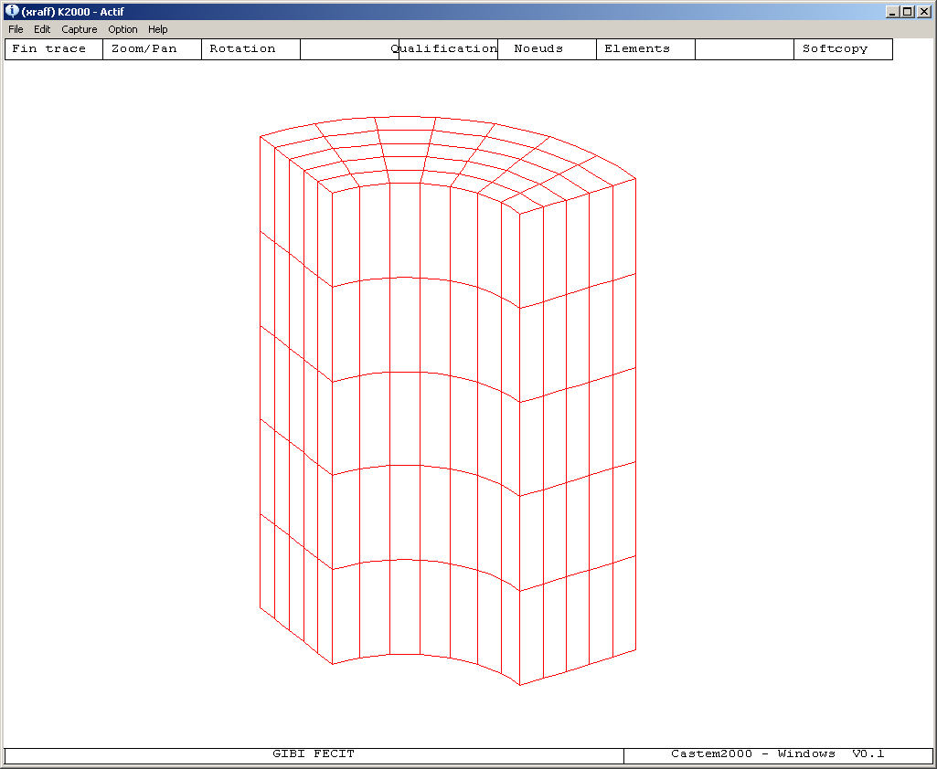
Figure 4.5-b: Meshing of the quarter cylinder considered (SSNV124) .
4.6. Comparison of limit analysis and incremental elastoplastic calculation up to ruin on an example#
We know that in perfect elastoplasticity, the tangent operator has zero eigenvalues from a certain level of force loading: this means that the elastoplastic solid has reached plastic ruin.
It may be interesting to perform an elastoplastic calculation (with von Mises criterion) incremental to the point of failure, in order to obtain a lower « limit » of the limit load. As the Newton algorithm used to solve the nonlinear static equilibrium diverges for this level of loading, it is necessary to use control by arc length [R5.03.80], or on a displacement variable, used to control the loading by the deformation of the solid undergone before the ruin.
Here is an industrial example: this is the calculation of the internal pressure limit of a Canopy tank joint. The problem is axisymmetric; the room is stuck on its upper border. The resistance limit (fixed rate) is set at \(100\mathit{MPa}\); a vonMises criterion is accepted. Two calculations were carried out:
a limit analysis calculation using the method presented in the preceding paragraphs;
a perfect elastoplastic incremental calculation (without and with work hardening), with the VONMise criterion in large transformations (Simo-Miehe, see [R5.03.21]), in order to verify that the change in geometry does not substantially modify the prediction of limit pressure.
limit analysis calculation |
elastoplastic incremental calculation in large transformations (Simo-Miehe) |
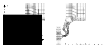
Figure 4.6-a. Deformed mesh (amplified)
The [Fig. 4.6-a] shows that the calculated deformations are very similar between the two methods and make it possible to predict the mode of ruin.
The [fig. 4.6-b] shows the convergence of the sequences of the limit pressure terminals \({\underline{\lambda }}_{m}\) and \({\stackrel{ˆ}{\lambda }}_{m}\) according to the regularization coefficient of the limit analysis calculation method, towards the exact limit pressure. The arithmetic mean of the two terminals seems to be a good estimate of the limit pressure. For the last value of the regularization coefficient chosen, we obtained the values reported in [tab.4.6-a]. They are compared with the perfect elastoplastic incremental calculation in large transformations. It can be seen that the values are very similar.
limit analysis: lower bound |
limit analysis: upper bound |
perfect elastoplastic incremental calculation |
\(\mathrm{18,72}\mathit{MPa}\) |
|
|
Table 4.6-a: Limiting pressures.
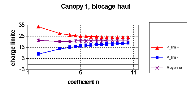
Figure 4.6-b. Limit analysis calculation: convergence of sequences \({\underline{\lambda }}_{m}\) and \({\stackrel{ˆ}{\lambda }}_{m}\) as a function of the regularization coefficient, towards the exact limit pressure.
The perfect elastoplastic incremental calculation in large transformations was carried out with two types of control:
by a radial displacement of a particular point;
by arc length (the latter control having been more efficient in terms of calculation time);
and the results were compared with those obtained by calculating in small transformations.
Finally, one of the questions that arises is the effect of the hardening of the material, and therefore of the choice of the resistance threshold.
This is why an incremental elastoplastic calculation was carried out taking into account the tensile curve of the material in question (the main parameters being: \({\sigma }_{y}\mathrm{=}195\mathit{MPa}\), \({\sigma }_{u}\mathrm{=}520\mathit{MPa}\)).
The [Fig. 4.6-c] allows us to note that in this case the two controls give an identical solution in large transformations, which is more « flexible » than in small transformations. The ruin pressure found is greater than \(\mathrm{56,4}\mathit{MPa}\). Reported for a value \({\sigma }_{y}\mathrm{=}100\mathit{MPa}\), we would have « found »: \(\mathrm{28,9}\mathit{MPa}\).
This example therefore makes it possible to gauge the conservative effect of the limit analysis method by having taken the elasticity limit as a resistance threshold \({\sigma }_{y}\) **.On the other hand, taking the ultimate limit* \({\sigma }_{u}\) as a threshold seems non-conservative, the structure undergoing substantial geometry changes as soon as it plasticizes, before ruin, in the path considered for the incremental calculation.
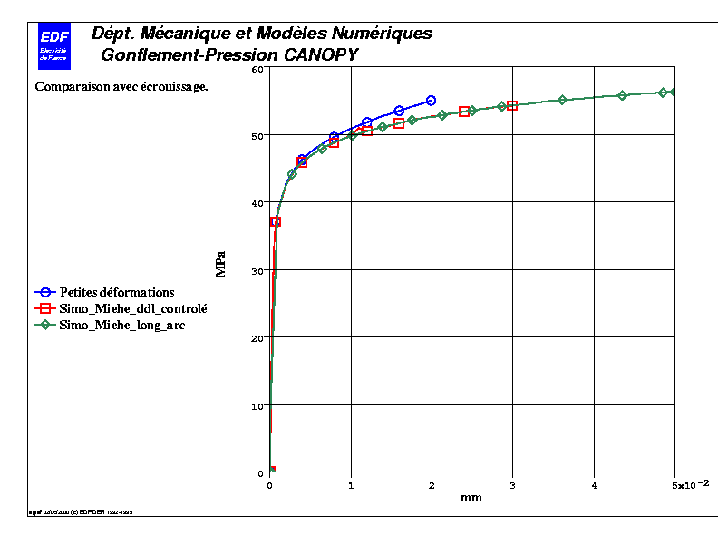
Figure 4.6-c. Incremental elastoplastic calculation in large transformations (Simo-Miehe) with two types of control, compared with a calculation in small transformations.