2. The main lines of the method#
2.1. Presentation#
The objectives of the boundary analysis are:
security analysis in the face of extreme behavior (Ultimate Limit State E.L.U.);
rapid sizing without trying to describe the entire ruin process;
the energetic characterization of ruin and the understanding of the modes of ruin;
obtaining simple information on the non-linear evolution of the material of the structure.
Boundary analysis is a problem that can be addressed in two ways, cf. [8], [9], [10]:
calculation of the « plastic » ruin of elastoplastic structures with a ductile plate. The loading path and the material behavior model should be fully described;
calculation of the loss of equilibrium potentiality using a given resistance criterion, for a given direction of loading. This is an optimization problem (under stress) of the load parameter \(\mathrm{\lambda }\). This approach is called « breakup calculation. »
For standard materials, these two methods give the same result.
The « fracture calculation » or « limit analysis » (term designating the fracture calculation in the case of an elastoplastic material with a normal flow rule) aims to determine directly, in a simplified manner and without resorting to the description of the loading path by an expensive elastoplastic incremental calculation, the boundary of the plastic ruin domain (and by deduction the domain of bearable loads) for a structure \(\Omega\), of geometry and limits resistance of the given materials, subject to a loading given by its direction \(\text{F}\), and whose amplitude is parameterized by the positive real \(\lambda\). A « permanent » load \({\text{F}}_{0}\), such as gravity, may possibly be present in addition (without being amplified by \(\lambda\)).
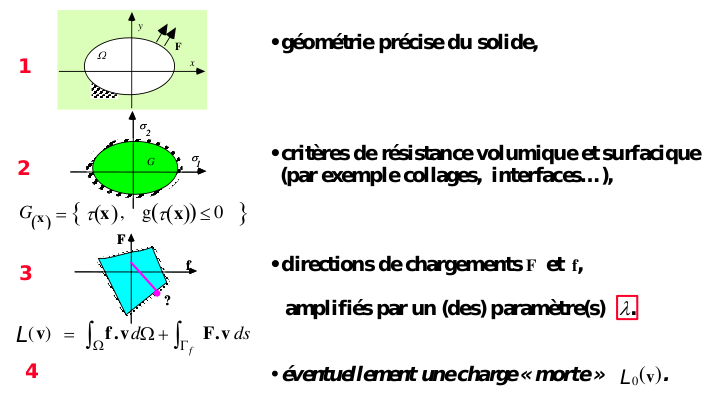
Figure 2.1-a: Ingredients of fracture calculation.
**Note: any change in geometry cannot be taken into account by the fracture calculation, as happens during a buckling failure, or for a very flexible solid This constitutes the hypotheses of the method: the configuration of the solid is that of it* initial geometry, the connections of the structure are assumed to be given and fixed until the ruin; similarly the loads, in force only, are of fixed directions.
Two approaches to fracture calculation are available:
the static approach that estimates the limit load value from the inside and requires the construction of statically admissible stress fields, which is difficult in general using finite elements. It consists in maximizing the loading parameter (s) provided that the (linear) static equations remain verified and that the constraint criterion is not violated;
the kinematic approach, which is dual to the previous one, which estimates the limit load value from the outside and which requires minimization by a method of regularizing the loading parameter (s) under the condition that the power of the external forces remains greater than the resistant power, (defined from the resistance criterion), of a non-regular functional, which must therefore be regulated in the general case.
Combined employment (ideal case!) of these two approaches provides limit load frameworks.
2.2. An analytical example [7]#
We consider a hyperstatic system with three bars: see [fig. 2.2-a], the bars have an identical resistance criterion, expressed in terms of normal effort (or tension) \(N\): \(g(N)=\mid N\mid \le \stackrel{ˉ}{N}\).
Point \(D\) is subject to a force \(\overrightarrow{F}\) with non-zero components \(({F}_{x},{F}_{y})\), amplified by a multiplicative factor \(\lambda\).


Figure 2.2-a: on the left: three-bar system; in the middle: domain of bearable tensions; on the right domain of bearable loads.
The space of statically admissible solutions (the tensions \({T}_{i}\) in the bars) is defined by the equations:
For positive \(\mathrm{\lambda }\), we see that it is in \({T}_{1}={T}_{2}=\stackrel{ˉ}{N}\) that the extremum is reached, see [fig. 2.2-a]. We thus find that the maximum bearable value of load factor \(\mathrm{\lambda }\) (or limit load), obtained by the static approach, is:
The kinematic approach gives the same result [6]: it is indeed the limit load of this problem.
2.3. Some useful properties of limit load calculation#
In the ideal case, the upper and lower limits of the limit load should be equal to the limit value. With the numerical approach, we will always have a gap and it is the lower bound that is the most penalizing. However, it should be noted that, for structures whose calculation can be carried out sufficiently far (as in test cases), the upper bound is in practice the one that is closest to the exact value.
The elastic limit is frequently chosen as the resistance threshold: this is in the direction of safety.
Some useful properties of limit load calculation are mentioned below (see [4], [8]):
the limit load is proportional to the value of the resistance limit or threshold \({\sigma }_{y}\) in a homogeneous solid. It does not depend on the history of the load undergone by the structure beforehand;
as the resistance criterion is convex (vonMises criterion), the domain of bearable loads (therefore the boundary of limit loads) in the load space is convex. It is therefore possible to approach the domain of admissible loads by the generalized polyhedron built on the vertices, each corresponding to a direction chosen in the load space;
the Dirichlet conditions (an imposed displacement) that are applied to part \({\Gamma }_{u}\) of the edge \(d\Omega\) of the structure, or an initial anelastic deformation —thermal, plastic… — have no effect on the range of admissible loads, (since ruin is the impossibility of satisfying the balance, the mode of ruin corresponds to a speed and direction of flow);
the limit load does not depend on the possible presence of a field of self-balanced stresses (residual stresses);
for a two-dimensional solid, the material and the direction of loading being given, a**lower**bound obtained by the static approach in**planar constraints**is necessarily lower than the exact limit load obtained in**plane deformations*: \({\mathrm{\lambda }}_{{C}_{\text{PLAN}}}^{-}\le {\mathrm{\lambda }}_{{D}_{\text{PLAN}}}^{\text{lim}}\);
conversely, an**upper limit**obtained by the kinematic approach in**plane deformations**is necessarily lower than the exact limit load obtained in**plane constraints*: \({\mathrm{\lambda }}_{{D}_{\text{PLAN}}}^{+}\ge {\mathrm{\lambda }}_{{C}_{\text{PLAN}}}^{\text{lim}}\). This result therefore provides a boost. If it is desired to treat a problem with plane stresses, it is then necessary to do the kinematic approach on a three-dimensional modeling of a « slice » of solid;
the limit loads obtained in plane deformations with the Tresca criterion are worth \(\sqrt{3}/2\) times those found with the von Mises criterion;
with a given geometry and direction of loading, if we replace in a given area of the structure the material with resistance domain \({G}_{1}\) by a material with resistance domain \({G}_{2}\subset {G}_{1}\) (\({g}_{2}(\tau )\le {g}_{1}(\tau )\)) (for example: Tresca criterion included in that of von Mises), then the support functions (maximum resistant powers) are: \({\mathrm{\pi }}_{2}(\mathrm{\varepsilon }(v))\le {\mathrm{\pi }}_{1}(\mathrm{\varepsilon }(v))\) and therefore: \({\mathrm{\lambda }}_{2}^{\text{lim}}\le {\mathrm{\lambda }}_{1}^{\text{lim}}\);
in particular if we replace a defect \(1\) (hole, crack) present in the structure by the defect \(2\) containing the defect \(1\), then we have: \({\lambda }_{2}^{\text{lim}}\le {\lambda }_{1}^{\text{lim}}\). Likewise, if the structure is heterogeneous, with two zones whose resistance limits are \({\mathrm{\sigma }}_{\mathrm{y1}}\le {\mathrm{\sigma }}_{\mathrm{y2}}\), the limit load will be greater than that of the same homogeneous situation for threshold \({\mathrm{\sigma }}_{\mathrm{y1}}\) and less than that for threshold \({\mathrm{\sigma }}_{\mathrm{y2}}\);
in the presence of a loading direction \(f=\lambda (\alpha {f}_{1}+(1-\alpha ){f}_{2})\) combining two directions \({f}_{1}\) and \({f}_{2}\), \(\mathrm{\alpha }\in \left[\mathrm{0,}1\right]\), then the exact load limit checks: \({\lambda }^{\text{lim}}(\alpha )\ge \stackrel{ˉ}{\lambda }=\frac{{\lambda }_{1}^{\text{lim}}{\lambda }_{2}^{\text{lim}}}{(1-\alpha ){\lambda }_{1}^{\text{lim}}+\alpha {\lambda }_{2}^{\text{lim}}}\). This result remains valid for approximations within the limit loads.
While general three-dimensional situations are unaffordable analytically, in 2D plane deformations (D_ PLAN) and plane constraints (C_ PLAN) it is possible to manually build and calculate solutions for the static approach and the kinematic approach, using fields built in blocks, which give frames for the limit load: this is useful to corroborate a result obtained by finite elements.