3. The implementation of boundary analysis#
3.1. The calculation steps#
To perform a limit analysis, you must:
use a 2D (plane or axis) or 3D mesh compatible with incompressible finite elements;
define the model with the incompressible finite elements;
define the strength limit of material \({\sigma }_{y}\);
define permanent loading \({\text{F}}_{0}\) and variable loading \(\text{F}\) which is driven by \(\mathrm{\lambda }\);
define the incompressibility condition;
perform a non-linear calculation with the incremental behavior and control provided for the limit analysis;
post-process the calculation to obtain the upper and lower values of the estimated load limit.
3.2. Meshing#
For the choice of mesh and the use of incompressible elements, refer to the documentation [R3.06.08]
Note: the use of a three-field element UPG will require*impose a boundary condition on the swelling (GONF), so the vertex nodes must be perfectly identified in the mesh:*
or as early as the design and production of the mesh;
or, more simply and retrospectively, by using the command DEFI_GROUP [:external:ref:`U4.22.01 <U4.22.01>`] with the keyword CREA_GROUP_NOen specifying the group of elements of incompressible elements and using the option* ** CRIT_NOEUD = “SOMMET” . *
3.3. Model#
3.3.1. Modeling options#
Incompressible elements must be selected, so we refer to the command AFFE_MODELE [U4.41.01].
3.3.2. Incompressibility condition#
To express the incompressibility condition for incompressible elements UPG with three fields, we use the command AFFE_CHAR_MECA [U4.44.01] with the keyword DDL_IMPO to require the GONF component of the group of vertex nodes of the incompressible elements to remain zero.
3.4. Material#
The material used for limit analysis with incompressible elements is a material with a von Mises criterion, an elastoplastic that is perfectly plastic.
Material characteristic data is provided under the keyword factor ECRO_LINE from command DEFI_MATERIAU [U4.43.01].
The slope of the traction curve (\({E}_{T}\)) is chosen to be zero (operand D_ SIGM_EPSI), the only data required to be provided is therefore the elastic limit (i.e. the resistance threshold in our case) (operand SY).
3.5. Loading#
The variable load \(\text{F}\) which is controlled by \(\mathrm{\lambda }\) must necessarily be of the effort type (force, pressure, gravity) and declared in the command AFFE_CHAR_MECA [U4.44.01].
If the structure is also subject to a loading process \({\text{F}}_{0}\), remember to remember this during post-processing (see [§ 3.8]).
3.6. List of moments#
The list of moments is used to control the Norton-Hoff regularization method, cf. [1], [5], by means of a coefficient \(m\), and not the evolution of the load as during an ordinary calculation:
so that, when the instant becomes large enough, \(m\) tends to 1, and the behavior approaches perfect rigid-plastic behavior, see the uniaxial curve [fig. 3.6-a].
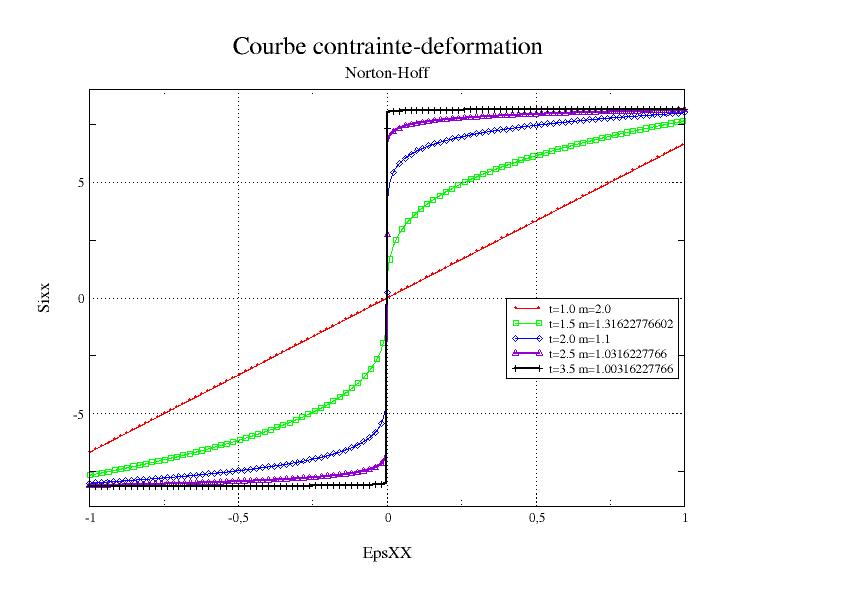
Figure 3.6-a. Stress-strain curve for various values at the moment \(t\)
In practice, a list of moments with constant steps will be chosen at the beginning (see Table 2.6-a) before refining the calculation steps in case of non-convergence.
1.0 |
1.5 |
2.0 |
2.5 |
3.0 |
… |
|
2.00 |
1.30 |
1.10 |
1.03 |
1.01 |
||
If the document for using the POST_ELEM command with the keyword CHAR_LIMITE [U4.81.22] recommends, in practice, to limit yourself to moments between 1 and 2 in order not to have calculations that are too long while making it possible to obtain a sufficiently accurate upper limit of the load limit, we observe that the lower limit load requires at least 2 to 3 additional iterations (instant greater than 3) to converge to the reference values in cases where tests.
3.7. Calculus#
Modeling with incompressible elements must use the STAT_NON_LINE [U4 *.* 51.03] command and the COMPORTEMENT keyword.
For limit analysis, it is mandatory to use the following operands of the STAT_NON_LINE command:
In COMPORTEMENTon choose RELATION =” NORTON_HOFF “ This operand is used to describe the viscosity behavior relationship (independent of temperature) in the calculation of limit loads of structures, at the von Mises threshold [:ref:`U4.*51.11 <U4*.* 51.11>`]
In PILOTAGE, we choose TYPE =” ANA_LIM “.This control mode is specific to the calculation of limit load (law NORTON_HOFF) using a kinematic approach. It should only be applied to the load declared using the keyword factor EXCIT, operand TYPE_CHARGE =” FIXE_PILO “.
Calculating the load limit can require a lot of linear search iterations and Newton iterations. It is therefore also strongly recommended to use the various calculation options in command STAT_NON_LINE to improve convergence, such as linear research, which practice shows that it is sufficient to use 2 or 3 iterations.
**Note: If we amplify the load intensity* \(L\to \mathrm{\beta }L\) (while we do not consider a permanent load \({L}_{0}=0\) ), the solutions depend on the factor \(\mathrm{\beta }\) according to the following relationships:
: label: EQ-None
{u} _ {m} (beta) = {beta} = {beta} ^ {-1} {1} {u} _ {m} (beta)) = {beta}) = {beta}) = {beta} ^ {1-m} {sigma} ^ {D} ({u} _ {m} (1))
At convergence for \(m\to {1}^{+}\), the load limit given by solution \({u}_{m}(\mathrm{\beta })\) is indeed the same as that given by \({u}_{m}(1)\), since \({\lambda }_{\text{lim}}(\beta )={\lambda }_{\text{lim}}(1)/\beta\).
3.8. Post-treatment#
From the result of the nonlinear calculation carried out, the operator POST_ELEM [U4.81.22] and the keyword CHAR_LIMITE produce a table that gives, for each moment of the calculation, the estimate of the upper bound CHAR_LIMI_SUP (\({\stackrel{ˆ}{\lambda }}_{m}\)) of the limit load supported by the structure; this sequence is monotonic decreasing when \(m\to {1}^{+}\), that is to say when \(t\to +\infty\).
In addition, in the absence of a permanent load \({F}_{0}\) (operand CHAR_CSTE =” NON “which is the default option), the table also contains the estimate CHAR_LIMI_ESTIM (\({\underline{\lambda }}_{m}\)) of the lower bound of the limit load. This value (approximation of the resistance convex gauge) is only calculated at the Gauss points of the finite elements. Therefore, the value \({\underline{\lambda }}_{m}\) obtained for each \(m\), less than \({\stackrel{ˆ}{\lambda }}_{m}\) [6], can only be considered as an indication (this sequence is not necessarily monotonic). With the excess value \({\stackrel{ˆ}{\lambda }}_{m}\), it makes it possible to provide a framework for the limit load of the discretized problem.
On the other hand, if a permanent load \({F}_{0}\) is present (operand CHAR_CSTE =” OUI “), such an estimate of the lower bound is no longer available and the table then indicates the power PUIS_CHAR_CSTE of the constant load in the speed field solution of the problem.
The visualization of the displacement field obtained for a value of the coefficient \(m\to {1}^{+}\) gives an « idea » of the ruin mode of the structure under study. More details on post-processing can be found in [R7.07.01].