3. Resolution#
3.1. General diagram of the resolution algorithm#
3.1.1. Definition and general remarks#
What is called « contact resolution » is the operation consisting in solving the system formed by the juxtaposition of classical mechanical equations and contact/friction equations (the geometric aspect being treated by pairing, all that remains at this stage is the non-linearity of the friction threshold and the non-linearity of contact status).
It should be noted that the two formulations available in the code differ significantly on this point. Without going into details, we briefly explain these differences later.
While discrete and continuous formulations are equivalent to solving the same physical problem, as their name suggests, they do not formulate it numerically in the same way. The differences between these two formulations are presented in a synthetic manner.
Discreet formulation case.
In discrete formulation, the contact and friction conditions are applied to the discretized system thanks to Newton « sub-iterations ». In a typical Newton iteration, we have two steps: firstly, we calculate only the resolution of the linear system obtained by Newton \(\mathit{Ku}=f\) with the initial contact conditions, then, secondly, by various optimization methods under condensed constraints on the contact zone, we solve the conditions of contact inequalities. This second step makes it possible to recalculate the « true » contact pressures. For the next Newton iteration, the second member is modified so as to be able to take into account the new contact conditions resulting from the second step. For discrete penalization, matrix \(K\) is also modified to limit interpenetrations. This technique makes it possible to solve problems with low contact ddls in an efficient manner. It can be said that the discrete formulation algebraically imposes contact conditions without constructing a continuous element for contact.
Formulation case continues.
In continuous formulation, a mixed variational formulation is written to take the contact-friction equations. The variational formulation is of the classical Lagrangian type for method LAC, increased Lagrangian for method STANDARD and penalized Lagrangian for method PENALISATION. The approach adopted to solve the non-linear system is to create late continuous contact elements. These late contact elements carry master-slave displacement ddls as well as Lagrange multipliers only on the slave side. When DEFI_CONTACT is run, contact pairs are created transparently to the user allowing the ddls to be described according to the topology of the potentially contacting meshes. Likewise, at the time of the resolution in STAT_NON_LINE, continuous elements by contact pair are created which allow the calculation of elementary matrices and vectors that will be combined with the overall stiffness of the mechanical system. A typical Newton iteration therefore provides for each resolution movements but also Lagrange multipliers (LAGS_C). The main advantage of the continuous method is to propose, via the degree of freedom LAGS_C (in field DEPL), access to contact pressure on the slave surface. However, attention is drawn to the fact that this quantity is in fact only a contact force density per unit area expressed on the reference configuration. In particular, in large deformations, it can no longer be described as pressure because it no longer makes physical sense. Because of the size of the system, continuous formulation is often less efficient than discrete formulation but more robust and more qualitative in various situations (plasitcity+contact for example).
3.1.2. Discreet formulation#
To illustrate the definition in the preceding paragraph, the general diagram of the algorithm is given in the case of a discrete formulation. We can make the following remarks about this diagram:
it only represents a single time step, assuming that we place ourselves in small slips (we therefore do not make the external loop appear, as in the, dealing with geometric nonlinearity and described in § 2.4);
in this diagram, the three classical steps of a Newton’s iteration appear: assembly and resolution of the linear system, integration of the law of behavior, analysis of convergence;
the particularity of the discrete formulation of contact consists in**the adjunction**of an additional step between the resolution of the linear system (without contact) and the integration of the law of behavior.**This step can be thought of as post-processing the contactless system solution. **
The additional step carried out by the « discreet contact » box is aimed at the construction and then the resolution of the system increased by the contact and friction conditions. Two approaches exist to formulate discrete friction-contact conditions:
Writing a Lagrangian and dualizing the contact/friction conditions, we then artificially increase the size of the global system to be solved and we use an optimization algorithm to satisfy the constraints inequalities. This approach is covered in § 3.2.1.
penalization (or regularization) of the contact and friction conditions, we keep the same size for the global system but we enrich the matrix, there is no specific algorithm, it is the Newton algorithm that ensures convergence. On the other hand, the contact is only resolved approximately and the user must provide one or more parameters to control the algorithm. This approach is covered in § 3.2.2 and § 3.3.2.
What the « discrete contact » box produces at the output is a field of displacement verifying the conditions of touch-friction as well as of touch-friction reactions. These reactions are used in checking balance.
The discrete formulation is therefore based on the resolution of a mechanical problem without contact, which has an important consequence: we cannot simply treat the case of a structure where contact as well as friction participate directly in the blocking of rigid body movement (cf. § 4.4).
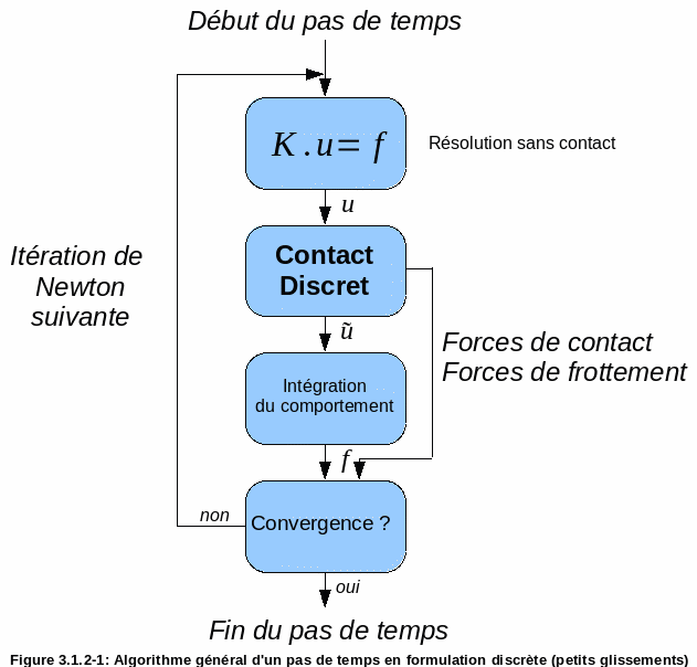
Figure 3.1.2-1: General algorithm of a time step in discrete formulation (small slips)
3.1.3. Continuous formulation: case ALGO_CONT =” STANDARD “/” PENALISATION “#
The general algorithm for resolving touch-friction with a continuous formulation is given, this one differs significantly from the diagram in discrete formulation. While with the latter the touch-friction is solved by sub-iterations (in the « Discreet Contact » box), the continuous formulation is based on a decoupling of non-linearities:
the non-linearity of friction (the Coulomb threshold depends on the contact pressure, which is itself an unknown) is treated by a fixed point on the value of the contact multiplier or a generalized Newton algorithm
contact nonlinearity is based on a status algorithm (with packet switching) or a generalized Newton algorithm
When all the non-linearities are decoupled, only the classical material and kinematic nonlinearities remain in Newton’s algorithm.
To formulate contact terms weakly, an increased or penalized Lagrangian is used, which makes it possible to regularize the initial non-differentiable system. Each Newton iteration in continuous formulation does not cost more in memory than in a contactless calculation of equivalent size in contrast to the discrete formulation. However, the nesting of loops or the treatment by the generalized Newton algorithm involve a greater number of iterations (Newton).
In continuous formulation, there are additional degrees of freedom in modeling, a consequence of the variational writing of contact conditions, as explained in § 4.3.2.
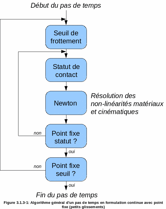
Figure 3.1.3-1: General algorithm of a time step in continuous formulation with a fixed point (small slips)
In continuous formulation, two algorithms exist to control variables specific to contact (internal variables by analogy to laws of behavior):
fixed point method on contact statuses: the status of contact statuses is evaluated in a loop external to the Newton loop. To choose the algorithm, use the global keyword ALGO_RESO_CONT =” POINT_FIXE “. The fixed point method (ALGO_RESO_CONT =” POINT_FIXE “) is the most robust but also the most expensive since the non-linear problem (plasticity for example) is solved with each change in contact statuses.
generalized Newton method: contact statuses are evaluated at each Newton’s iteration (this is the default). The generalized Newton method (ALGO_RESO_CONT =” NEWTON “) is more efficient but sometimes poses convergence problems. The ADAPTATION keyword makes this mode of convergence robust. In the event that we cannot agree on the statuses despite the ADAPTATION keyword, we must return to a fixed point method.
3.1.4. Continuous formulation: case ALGO_CONT =” LAC “#
This method makes it possible to resolve the pressures and the effects on the intersected contact cells in an averaged manner. It is part of the family of MORTAR methods that are renowned for their ability to deal with interface problems in mechanics. It only has meaning for each contact element. The problems associated with the exclusion of redundant nodes for the standard/penalized continuous formulation with boundary conditions is not a problem for this method since the contact conditions are not imposed on the nodes but on a per element basis.
The LAC (Local Average Contact) method does not use a fixed point loop. All contact nonlinearities (status+geometry) can vary from one Newton’s iteration to the next. Only convergence criteria make it possible to control the quality of contact resolution. At the moment the LAC method does not yet solve the friction.
Finally, to use method LAC, it is necessary to carry out a mesh pre-treatment phase (CREA_MAILLAGE/DECOUPE_LAC) which consists in preparing the slave « patches » for the contact conditions verified by macro-mesh.
3.1.5. Continuous formulation: treatment of incompatibilities.#
In the case of meshes where the incompatibility is low, standard/penalized continuous methods can be used. To realize the influence of mesh compatibility, under the keyword ZONE of DEFI_CONTACT, you can activate a keyword that reduces contact pressure oscillations: INTEGRATION. However, the keyword has two drawbacks: the number of active contact statuses is not available at the end of each calculation increment and there is also no CONT_NOEU at the end of the calculation. So you have to fall back on post-processing with CALC_PRESSION. In the case of strong mesh incompatibilities, method LAC makes it possible to have a good quality of contact pressures.
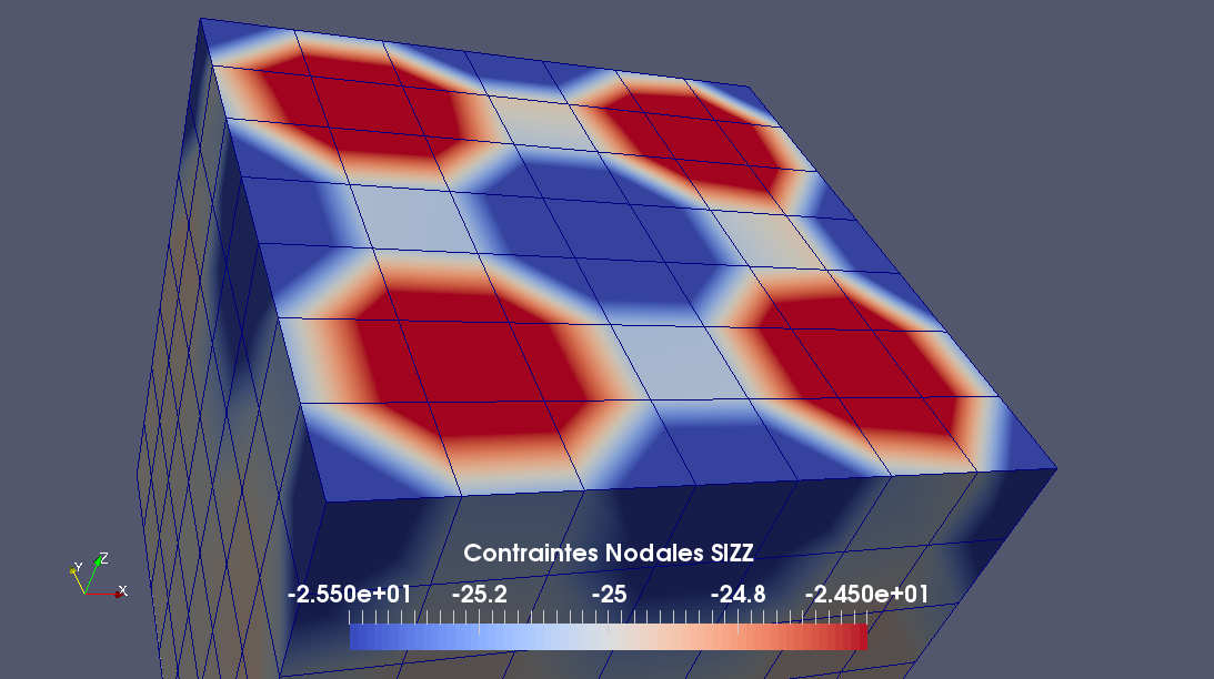
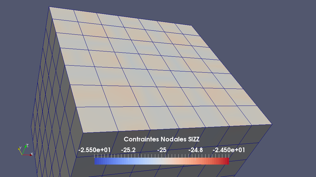
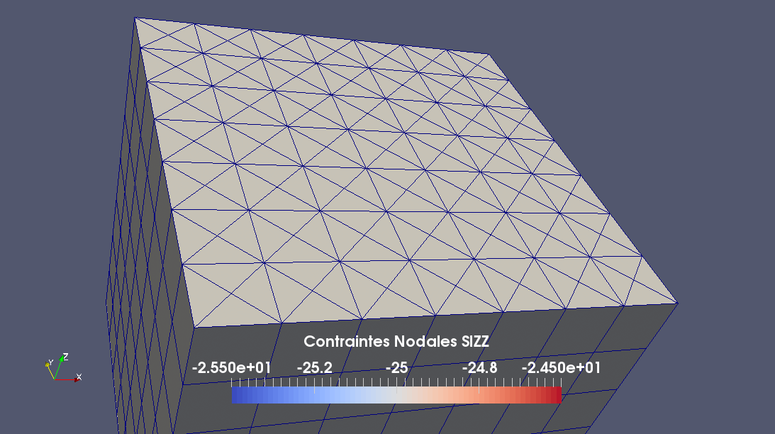
On the example of the analytical test case « Taylor patch test » SSNP170 (contact between two parallelepipedic blocks with analytical pressure of -2 5MPa), we note that depending on the configuration of the integration of the contact terms, depending on the configuration of the integration of the contact terms, the oscillations disappear or not.
Integration type |
Visualization of nodal constraints |
AUTO |
|
NCOTES |
|
LAC |
|
3.2. Solving a problem with contact alone#
3.2.1. Dualization in discrete formulation (FORMULATION =” DISCRETE “)#
3.2.1.1. Principle#
The dualization of the discrete system consists in the introduction of a Lagrangian (cf. [R5.03.50]). The system to be solved takes the following form when it is reduced to the active links:
Knowing that the resolution of the contactless system has already been carried out, the solution for the following system is known:
The resolution technique is then based on the use of the system’s Schur complement to transform the system:
The problem transformed in this way is the size of the number of slave nodes and is full. Two algorithms to choose from are available to deal with this new problem:
an active constraints method (ALGO_CONT =” CONTRAINTE “) based on the**explicit construction** and the factorization of the Schur complement
a projected conjugate gradient method (ALGO_CONT =” GCP “) based on the**iterative** resolution of the system formed by the Schur complement of the system
Note that dualization requires the use of a direct linear solver: in*Code_Aster*, this means” MULT_FRONT “or” MUMPS “.
Each of the 2 algorithms mentioned above in fact carries out sub-iterations during which it is necessary to solve the linear system with \(C\) the stiffness matrix of the global non-contact system (which is much faster if \(C\) is already factored).
3.2.1.2. Method “CONTRAINTE”#
Based on factorization (therefore a direct solver) to solve the system associated with the Schur complement, the “CONTRAINTE” method does not require any parameterization. Moreover, its convergence [3]_ is demonstrated, which explains why it is the default method in the presence of contact.
However, the use of a direct solver has a major drawback: this algorithm is not suitable as soon as the number of slave nodes exceeds a few hundred (500). In fact, the factorization of a full matrix very quickly becomes prohibitive.
The construction of the Schur complement can be accelerated by using the parameter NB_RESOL (cf. [U4.44.11], by default value 10) at the expense of the memory consumed (the greater the total number of degrees of freedom, the more expensive it is to increase this parameter). In order to optimize a calculation with the active constraints method, it is advisable to perform a calculation on a time step in order to find a time/memory compromise (cf. [U1.03.03] for reading information on the memory consumed).
3.2.1.3. Method “GCP”#
When you can no longer use the default contact method because it is too expensive, an alternative is to use the “GCP” method. As mentioned above, this method consists in applying an iterative solver (projected conjugate gradient) to solve the dual problem.
The main advantage of such a method is to no longer be limited in size of problem (several thousand slave nodes are perfectly reachable). The counterpart, specific to any iterative solver, is a mandatory configuration for the user.
This method can be used in parallel computing, it is also the only discrete method to really benefit from it.
Like any iterative solver, the “GCP” method uses a convergence criterion: it is a criterion on the value of the game. Given by the RESI_ABSO keyword, it controls the maximum tolerated interpenetration.
It is mandatory and is expressed in the same unit as that used for meshing. It is recommended to first use a criterion equal to \({10}^{\mathrm{-}3}\) times the average interpenetration when the contact is not taken into account (see § 4.8).
If there are difficulties in the convergence of the projected conjugate gradient algorithm, there are 2 parameters on which it is recommended to play (additively, i.e. one then the other):
use an inadmissible linear search (RECH_LINEAIRE =” NON_ADMISSIBLE “)
use a Dirichlet pre-conditioner (PRE_COND =” DIRICHLET “)
The preconditioner has the advantage of being optimal and therefore significantly reduces the number of iterations necessary for convergence. In addition, when one is close to the solution, it makes it possible to reduce the residue very quickly and therefore to achieve very low interpenetration criteria.
Its disadvantage is a significant cost that can often prevent a gain in calculation time despite the reduction in the number of iterations.
For this reason, it is possible to request its activation only when the residue has sufficiently decreased: the pre-conditioner then ideally makes it possible to converge in a few iterations. The difficulty lies in quantifying the « sufficiently reduced » or in other words the proximity of the solution. This triggering is controlled by the keyword COEF_RESI, which is the coefficient (less than 1) by which it is necessary to have multiplied the initial residue (the initial maximum interpenetration therefore) before applying the preconditioner. An example of implementing this parameter is given in test case SSNA102E.
3.2.2. Penalization in discrete formulation: algorithm “PENALISATION”#
Penalization consists in regularizing the contact problem: instead of trying to solve exactly the conditions on the game and the pressure, we introduce a univocal approach which implies that we will always observe interpenetration when contact is established.
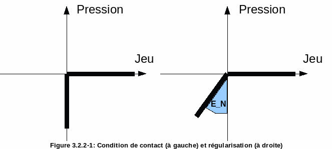
Figure 3.2.2-1: Contact condition (left) and regularization (right)
As shown, we add a parameter E_N to regularize the contact condition: the larger it is, the more we tend to the exact condition, the smaller it is, the more we tolerate interpenetration.
In discrete formulation, the concept of contact pressure does not exist because we reason about the nodes of the finite element mesh: we therefore work with nodal forces (cf. § 4.3). The so-called penalty coefficient E_N therefore has the dimension of stiffness (\({\mathit{N.m}}^{\mathrm{-}1}\)).
An analogy is generally made between the penalty coefficient and the stiffness of unilateral springs that would be placed between the master and slave surfaces where interpenetration is observed.
E_N is generally chosen by successive tests:
first of all, we will start by taking a value equal to 10 times the largest Young’s modulus of the structure multiplied by a characteristic length of the structure;
if the calculation gives a result (satisfactory or not), the value will then be increased by multiplying it by 10 each time until a stable result is obtained in terms of movements and especially in terms of constraints.
The advantage of the penalization method is not to increase the size of the system contrary to dualization, but also to not restrict the choice of the linear solver. The downside is a sensitivity to the penalty coefficient, which implies systematically conducting a parametric study before embarking on long calculations (cf. [U1.04.00] and [U2.08.07] for the launch of distributed parametric calculations).
To help calibrate the penalty coefficient, there is an automatic adaptation mechanism based on the DEFI_LIST_INST [U4.34.03] command. An example of implementation can be found in test case SDNV103I [V5.03.103].
3.2.3. Formulation “CONTINUE”: advice on solvers and parallelism#
For the problem of contact alone, the continuous method has the advantage, like the (discrete) method of active constraints, of not requiring any adjustment by the user.
In addition, as it is not dependent on a solver linear direct, it is possible to use an iterative linear solver (like “GCPC” or “PETSC”) to save a lot on calculation time. However, insofar as iterative solvers may prove to be less robust, it is advisable to turn to such a solver only once the computation with contact and friction has been developed and validated. In any case, it is strongly recommended to return to a direct solver in case of convergence difficulties.
When using an iterative solver with the continuous formulation of touch-friction , it is advisable to activate the Newton-Krylov method (cf.* **keyword METHODE de STAT_NON_LINE [U4.51.03]) which makes it possible to automatically adapt the convergence criterion of the linear solver ) which makes it possible to automatically adapt the convergence criterion of the linear solver . **
3.2.4. Other parallelism tips#
In case the user decides to use NORMALE =” ESCL “/” MAIT_ESCL “then, parallelism is not available.
In case of use of implicit DYNA_NON_LINE + DEFI_CONTACT /continuous, we require that the distribution be centralized. For the formulations, discrete, we impose to use in AFFE_MODELE/DISTRIBUTION =” CENTRALISE “.
For discrete formulations, it is necessary to use AFFE_MODELE/DISTRIBUTION =” CENTRALISE “in/=””.
3.3. Solving a problem with friction#
3.3.1. Treatment of threshold nonlinearity#
In Code_Aster, the only available friction model is that of Coulomb (cf. [R5.03.50]). An additional nonlinearity must be treated in the presence of friction: this is threshold nonlinearity.
In fact, the friction threshold depends on the contact pressure, which is itself unknown.
Coulomb’s law involves a coefficient \(\mu\), called the Coulomb coefficient. During the so-called adhesion phase, a point in contact does not move (it has zero speed and there is a tangential reaction). During the sliding phase, the point has a non-zero speed and is subjected to a tangential reaction equal to \(\mu\) times the normal reaction.
In general, if the coefficient of friction is very low, it is advisable to neglect the friction. In addition, it is advisable in studies to treat initially only contact, in order to introduce non-linearities one after the other.
The discrete methods that they work by penalization or dualization rely on algorithms dedicated to the presence of friction (distinct from those used for contact) while the standard/penalized continuous method uses two different algorithms:
fixed point method on friction thresholds: the threshold is updated in a loop external to the Newton loop (and to the contact status loop); ALGO_RESO_FROT =” POINT_FIXE “.
generalized Newton method: the nonlinearity of friction is treated in the Newton process, by explicit derivation of all non-linear terms. ALGO_RESO_FROT =” NEWTON “.
3.3.2. Discreet formulation: penalization of friction (algorithm “PENALISATION”)#
For 3D or large problems, it is advisable to treat the friction problem by penalization. As with contact penalization, this requires the entry of a penalty parameter (E_T). More difficult to choose than its equivalent E_N, it requires a small parametric study to be carried out.
To make the analogy with the case of the penalization of contact, we will notice that the phase of adhesion itself disappears (as soon as the contact is activated there is interpenetration, in friction there is always sliding).
Convergence can also be accelerated by using the COEF_MATR_FROT keyword.
3.3.3. Formulation “CONTINUE”: STANDARD/PENALISATION.#
This is the method of choice when dealing with a touch-friction problem: it is the most robust and it also tolerates large friction coefficients (greater than \(\mathrm{0,3}\)) well.
It is possible to choose between two resolution algorithms to fix the internal variables specific to touch-friction with the keyword ALGO_RESO_XXXX (XXXX = CONT/FROT).
The fixed point method (ALGO_RESO_XXXX =” POINT_FIXE “) is robust but expensive. The generalized Newton method (ALGO_RESO_FROT =” NEWTON “, choice by default) is very efficient and offers a good level of robustness. The big advantage of this algorithm is its lower dependence on the value of the coefficient of friction, since there is no loop on the thresholds. A non-symmetric tangent matrix is produced, which represents a slight additional cost during factorization and limits the range of iterative solvers that can be used.
It is preferable to use the generalized Newton method since the coefficient of friction is not negligible. The savings in calculation time are very significant (up to 80% gain compared to the fixed point).
The two algorithms” POINT_FIXE “/” NEWTON “give identical results.
However, when convergence difficulties occur, in particular in the presence of significant slippage, the user can set the coefficient COEF_FROT (which has the dimension of the inverse of a distance). This parameter takes a value of 100 by default: we will try values between \({10}^{-6}\) and \({10}^{6}\). For studies where adherence is predominant, values of COEF_FROT that are lower than the default value will be preferred while for cases where slippage is predominant, higher values will be chosen. There are alternatives to the hard setting of COEF_CONT or COEF_FROT: these are the adaptive methods.
A first backup solution is to favor the method of continuous penalization with adaptive methods (ALGO_CONT =” PENALISATION “/ ADAPTATION =” TOUT “). Indeed, it is possible to activate an algorithm for automatically controlling the penalty coefficient (via cycle analysis). If we only want to control the penalty coefficient without contact statuses then we will use the keyword ADAPTATION =” ADAPT_COEF “. This method may fail in the sense that the control may not be effective, but it will only affect the speed of convergence and not on the quality of the results. Alternative options exist to get around the problems of convergence with friction:
Activate the exact contact resolution and the penalized friction resolution and initially limit the number of geometric updates: ALGO_RESO_GEOM =” CONTROLE “, ZONE/ALGO_CONT =” STANDARD “+ ALGO_FROT =” PENALISATION”.
In case the technique above did not work: consider using ADAPTATION =” TOUT “in the keyword ZONEpour to deal with both cycling and the adaptation of adjustment coefficients.
There is a mode that is activated as soon as the ADAPTATION keyword is active: it is FLIP - FLOP. It allows convergence to be declared in contact status as soon as the contact pressure is stabilized in the contact zone. This pressure is an arithmetic mean of the contact pressures of all zones.
3.4. Summary for choosing resolution methods#
3.4.1. For contact and friction#
For problems with a low number of degrees of freedom in contact (less than 1000 degrees of freedom), preference will be given to a discrete formulation with an active constraints algorithm (“CONTRAINTE”). If friction must be activated, we will use a “CONTINUE” formulation.
For problems with a large number of degrees of freedom in contact (greater than 1000 degrees of freedom), the iterative resolution algorithm using active constraints” GCP “is the most appropriate. However, if we have to take friction into account, we can turn once again to the formulation “CONTINUE”.
For large problems (regardless of the number of degrees of freedom in contact), the resolution of the linear system consumes a large part of the calculation time, so the choice of the linear solver is essential. The “CONTINUE” method is well suited in that it leaves it up to the user to choose the linear solver and that it is well parallelized.
3.4.2. For the linear system#
If a discrete formulation is used (excluding penalization), only direct linear solvers are accessible. We will therefore choose the solver “MULT_FRONT” unless we perform a parallel calculation in which case we will select “MUMPS”. The “GCP” method combined with the linear solver “MUMPS” benefits from a good level of parallelization in the contact algorithm.
If a continuous formulation is used, it is advisable, as soon as the global problem exceeds 100,000 degrees of freedom, to use an iterative solver associated with the “LDLT_SP” preconditioner and the Newton-Krylov method (see § 3.2.3). If the calculation involves friction or is parallel, the iterative solver “PETSC” is the best choice.