4. Methodologies#
In this section, questions frequently asked during contact friction studies are answered. The techniques implemented in this part often rely on operators other than DEFI_CONTACT, we will briefly describe the keywords to use, but the user can advantageously refer to the documentation for using these commands.
4.1. What to do when a contact calculation does not converge or does not converge to the right solution?#
Very often, convergence problems in contact have a physical origin and are not due to a problem of operator robustness.
The advice given below is only indicative. In practice, it is proposed to follow the following list:
Do not activate all nonlinearities at the same time. Always start by activating the contact alone in linear elasticity and see if it converges.
For very localized or occasional contacts, maybe DEFI_CONTACT is not the right operator (cf. AFFE_CHAR_MECA/LIAISON_MAIL, etc.).
For incompatible meshes, consider using method LAC or changing your mesh if possible.
For permanent contacts, the GLISSIERE keyword can be useful.
In case of failure to integrate the law of behavior, check that it is not due to a mesh flip caused by the touch-friction condition (cf. Figure).
- A converged calculation in the Newton sense is not necessarily a relevant calculation. It is up to the head of the study to take a critical look at the values obtained. From the viewpoint of contact, it is necessary to monitor monitor the presence of contact pressure oscillations, control the values of CONT_NOEU/CONT_ELEM. In the case of a penalization algorithm, you absolutely must look at the maximum penetration values visible in the convergence table. A mesh convergence study or the comparison of the solution with a reference result may be necessary to confirm the quality of the solution obtained.
- When a calculation has difficulty converging on status at a point of contact (in ALGO_CONT =” STANDARD “), the algorithm automatically suggests a switch to penalization resolution mode on the point that is having trouble converge. At the point that is having trouble converge. The penalty coefficient is chosen so as to limit interpenetration and the algorithm automatically switches back to the standard method as soon as convergence on status has been achieved. It is up to the user to check the quality of the result at the end of the calculation. If you want to unplug this mechanism, you must use ADAPTATION =” NON “ .
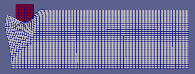
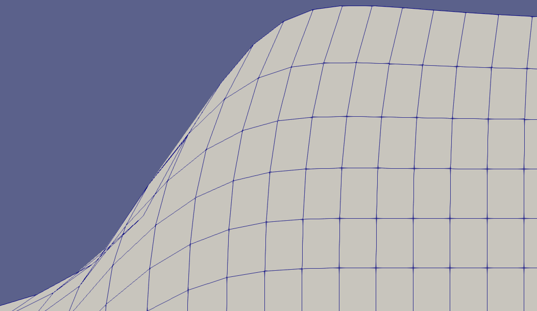
Figure 4.1-1: Flipped mesh situation leading to the failure to integrate the law of behavior
Sometimes the contact calculation converges in elasticity but poses a problem with material nonlinearity or large transformations. Generally, the nonlinear resolution algorithm has trouble when the solution calculated at the first Newton’s iteration (prediction) is too far from the real solution. In this case, one solution is to start the calculation with a predictive displacement close to the final solution. To do this, the easiest way is to do a first elastic calculation over one or two steps of time close to the moment of non-convergence. Then use the calculated elastic displacement as the predictor for the completely non-linear calculation: STAT_NON_LINE/NEWTON/PREDICTION = “DEPL_CALCULE”.
Use REAC_GEOM =” CONTROLE “very carefully and always check your result (visually and the convergence chart). Adaptive methods activated by the ADAPTATION keyword help with convergence but can do nothing against poor data layouts.
For calculations that require friction modeling. Start without friction first. Activate ALGO_RESO_FROT =” POINT_FIXE “to limit excessive variations in the Coulomb threshold.
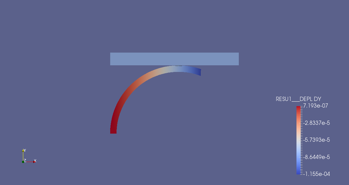
For calculations that only work through contact, the first advice is to use springs (DIS_T or 2D_DIS_T, see § 4.4). Another solution is to perform a first computation controlled while moving in order to initialize the contact and then to continue the calculation by forcibly controlling. This is the case in the figure below, where a first imposed displacement time step was taken to put the plate in contact with the ring and then the calculation was controlled while moving.
In terms of the quality of the solution, do not post-treat LAGS_C degrees of freedom directly. Prefer the fields contained in CONT_NOEU or CONT_ELEM or even those produced by the CALC_PRESSION command if the model allows it.
To check the quality of the solution, always check, using method STANDARD or PENALISATION, if the master stitches have not entered the slave meshes. In fact, in the so-called Node-Segment method, the master mesh does not have the same role as the slave mesh. Only the slave mesh strictly respects the law of non-interpenetration. In this case, it is because the mesh is generally too coarse. Remember to refine it (cf. § 2.2). Another tip is to multiply the number of slave contact points if you don’t want to step the mesh again (INTEGRATION =” NCOTES “, ORDRE_INT =6).
To check the quality of the solution, you have a diagnosis of the number of contact links that are actually active at the end of each time step. This may help to understand the mechanism being studied.
Number of contact links: 6
4.2. Post-processing of CONT_NOEU#
Field CONT_NOEU is generated when using the discrete or continuous formulation (with INTEGRATION =” AUTO “). In particular, this field contains vector quantities such as sliding forces (RTGX, RTGY, RTGZ), adhesion forces (RTAX, RTAY, RTAZ), normal forces (RNX, RNY, RNZ). They are always expressed in the global frame of reference but you can use MODI_REPERE to change it. For example:
RESU = MODI_REPERE (
RESULTAT = EVOLNOLI,
NUME_ORDRE = 1,
MODI_CHAM = (_F (NOM_CHAM = “CONT_NOEU”,
NOM_CMP =( “RNX”, “RNY”, “RNZ”,),
TYPE_CHAM = “VECT_3D”,),),
REPERE = “UTILISATEUR”,
AFFE = _F (ANGL_NAUT =( 45,45.0),),
4.3. Recover contact pressure#
4.3.1. Introducing CALC_PRESSION#
When post-processing a contact calculation, it is generally desired to access the touch-friction forces. More precisely, we want to know the normal and tangential stress on the edge of the solids in contact.
The continuous formulation of the contact gives direct access to an estimate of the touch-friction pressure, while the discrete formulations require approximating it by the stresses on the edge.
An example of implementation for both formulations exists in test case SSNP154 [V6.03.154]. CALC_PRESSION provides a printable contact pressure CHAM_GD in table format for example.
Contact pressure is written as:
where \(\underline{n}\) is the normal to the contact surface in deformed configuration and \(\sigma\) is the Cauchy stress tensor.
The box below shows how to calculate nodal contact pressure using CALC_PRESSION.
# contact pressure calculation: P_appr_f
P_appr_f= CALC_PRESSION (MAILLAGE = MESH,
RESULTAT = RESU,
GROUP_MA =( “Bottom_C”, “Top_B”,),
INST =1.0,);
For a calculation in large displacements, the normal must be calculated on the deformed configuration. To do this, you must enter the keyword GEOMETRIE =” DEFORMEE “.
In the example above, the formula from is used to explicitly calculate contact pressure. In the particular case where the edge on which the pressure is extracted is parallel to the axes of the coordinate system, the pressure is directly equal to one of the diagonal components of the Cauchy stress tensor (SIXX, SIYY or SIZZ). Right now, you can’t use CALC_PRESSION if there are structural elements in the model.
4.3.2. Case of continuous formulation#
In continuous formulation, field DEPL contains one or more additional unknowns:
LAGS_C represents the surface contact force density expressed on the reference configuration.
LAGS_F1 and LAGS_F2 represent the coordinates of a direction vector in the tangential plane. This vector with a norm less than or equal to 1 indicates the direction of sliding or adherence when friction is taken into account.
These quantities are defined at any point on the contact slave surface. We can therefore easily access the contact pressure. However, it should be noted that in large movements, initial and final configurations no longer being confused, the degree of freedom LAGS_Cn no longer has the meaning of pressure.
To access the surface density of the friction force (in both the adhesion and sliding phases), an additional calculation must be carried out: the norm of the direction vector in the tangential plane in fact gives the amplitude with respect to the friction threshold.
If we write \(\lambda\) the contact pressure then the friction force density \(\tau\) is written as:
In penalized formulation (ALGO_CONT =” PENALISATION “), the degrees of freedom of pressure continue to exist, so we can apply the above.
It sometimes happens that the contact pressure measured by this method presents oscillations, in particular for curved geometries. In this case, it is preferable to use CALC_PRESSION which calculates the contact pressure from the Cauchy stress tensor.
4.3.3. Discreet formulation#
In discrete formulation, no degree of freedom is added to the main unknowns. Since the contact problem is formulated on the discrete system, the possible Lagrange multipliers used do not even have the dimension of pressure but that of nodal forces.
This absence makes it necessary to calculate the Cauchy stress tensor on the edge of the surfaces in contact. So we have only one alternative: CALC_PRESSION.
4.4. Rigid body movements blocked by contact#
This paragraph only applies to static studies. In dynamics, rigid body movements are allowed.
In studies, contact can block the rigid body movements of certain solids (and cause them to deform). The initial failure to take this phenomenon into account will therefore lead to the singularity of the stiffness matrix (and therefore the impossibility of solving).
Discreet formulations are not suitable for initial consideration of contact, the carrying out of studies with solids only held by contact will therefore require an enrichment of the modeling in this case.
The continuous formulation makes it possible to naturally take account of initial contact and as such is therefore well suited to the study of mechanisms.
For studies in three dimensions, there are 6 possible rigid body movements: 3 translations, 3 rotations. For studies in two dimensions (models D_PLAN, C_PLAN), there are 3 rigid body movements: 2 translations and one rotation. Axisymmetric modeling (AXIS) is particular: there is only one rigid body movement, the translation along the \(\mathit{Oy}\) axis (axis of cylindrical symmetry).
When we notice the existence of rigid body movements in our modeling, we will always start by verifying that there are no symmetries in the structure and its loading. In fact, symmetry conditions make it possible to eliminate a large part of rigid body movements.
An example of blocking rigid body movements in continuous formulation (by CONTACT_INIT) and in discrete formulation (by springs) is available in test case SSNA122 [V6.01.122].
4.4.1. Continuous formulation#
In continuous formulation, initial contact is taken into account zone by zone with the keyword CONTACT_INIT. By default at the start of a calculation all the links with zero clearance (or interpenetrated) are activated (CONTACT_INIT =” INTERPENETRE “). The tolerance, to determine if a game is null or interpenetrated, is set internally in the program to \({10}^{\mathrm{-}6}\mathrm{\times }{a}_{\mathit{min}}\) where \({a}_{\mathit{min}}\) represents the smallest non-zero edge of the mesh.
It is possible to deactivate this automatic activation (CONTACT_INIT =” NON “). When doing non-linear calculations with repeat (i.e. with the ETAT_INIT keyword from STAT_NON_LINE), it is essential to use the default value (“INTERPENETRE”) in order to ensure a recovery from the true contact state (and not from a blank state).
Finally, if you want to initially glue all the contact surfaces regardless of the initial play, you can select CONTACT_INIT =” OUI “(this can be useful if the meshes are not perfectly in contact).
In all cases where an initial contact is declared, efforts will be generated: it is not a simple geometric reposition aimed at gluing the meshes.
Activating an initial contact blocks rigid body movements in the direction normal to the surface. If we want to take into account an initial adherent state in order to block the tangent direction, we can specify an initial contact threshold that is not zero via SEUIL_INIT. This parameter provides the initial value of the contact pressure (homogeneous at a surface force density). By default, if the calculation is the result of a chase then the value of the initial threshold is automatically reconstructed using the values of LAGS_C contained in ETAT_INIT/STAT_NON_LINE.
It should be noted that the use of an initial contact in continuous formulation also makes it possible to avoid non-convergence when a structure is subject only to movements. For example, when two solids that were initially in contact are pressed against each other by displacements (it is therefore a rigid body movement).
4.4.2. Discreet formulation#
In discrete formulation, it is necessary to manually block the movements of the rigid body of the offending solid by springs of low stiffness. By « weak » we mean small enough to generate only nodal forces that are negligible compared to the nodal forces used in the calculation.
The aim of the springs is to ensure that the contactless calculation is capable of rotating in linear mechanics (i.e. in operator MECA_STATIQUE or in STAT_NON_LINE once the contact conditions have been removed).
There are two approaches to adding springs:
add a spring of low stiffness at any point of the structure
add springs at well-chosen points to block the rigid body movements of the structure
The first approach has the advantage of genericity but can sometimes disturb the solution too much (regardless of the stiffness of the springs). In fact, such an approach amounts to adding a positive term to all the diagonal terms of the matrix that makes it invertible.
The second approach only adds springs where necessary. When there are points in the structure that will have a slight displacement (therefore to generate only a weak nodal force in the spring), this approach is more suitable.
To apply a spring in*Code_Aster*, you need to create POI1 meshes from knots. To do this, we use the CREA_MAILLAGE/CREA_POI1 operator. To use the first approach we will choose to create this group of elements over the whole structure (TOUT =” OUI “), while for the second approach, we will indicate the desired group of nodes. The newly created group of elements will be used to assign a “DIS_T” or “2D_DIS_T” model in AFFE_MODELE.
The characteristics of the spring are defined in operator AFFE_CARA_ELEM. By default, the stiffness values are entered in the global coordinate system. If, for example, we want to block the movement of a rigid body in a direction parallel to the axes of the global coordinate system, we will only define a non-zero stiffness in this direction. Below is an example of defining a stiffness for a 2D calculation in the DY direction.
RESSORT = AFFE_CARA_ELEM (MODELE =model,
DISCRET_2D =_F (CARA =” K_T_D_N “,
GROUP_MA =” SPRING “,
VALE =( 0.,1.0e-1,),),);
In cases where the direction to be blocked is not parallel to the axes, two alternatives are possible:
define stiffness in all directions
define stiffness in a local coordinate system. It is then necessary to define the orientation of this coordinate system (keyword ORIENTATION of AFFE_CARA_ELEM) or else use springs that no longer rely on POI1 but SEG2 meshes.
For an example of using springs, consult test case ZZZZ237 and its documentation [V1.01.237].
4.5. Large deformations, large displacements and contact#
Taking into account contact and friction conditions is completely decoupled from taking into account large displacements or large deformations. More generally, any non-linearity, regardless of material or geometric nature, is*a priori* compatible with the use of contact.
In practice, convergence difficulties are often observed in studies combining the three nonlinearities. The procedure to be adopted in this case is given in the rest of this section.
Examples of calculations combining the three nonlinearities are available in test cases SSNP155 [V6.03.155], SSNP157 [V6.03.157] and SDNV103 [V5.03.103].
For method LAC, it is possible to use TYPE_JACOBIEN =” ACTUALISE “instead of” INITIALE “in the case of large transformations.
4.5.1. Decouple nonlinearities#
When such a calculation fails, the first step is to go back: by decoupling the nonlinearities and by trying to apply good practices in a non-linear way (cf. [U2.04.01]).
That means:
perform an elastic calculation in small disturbances with the contact activated. If this calculation fails, apply the advice given in the first part of this document (orientation of normals, choice of master and slave surfaces, choice of the resolution algorithm,…)
perform a calculation with a non-linear but non-contact law of behavior. If this one fails, then the problem comes from integrating the behavior. We will then refer to the documentation [U2.04.02] and [U2.04.03].
if necessary, perform a calculation in large displacements but without contact and without material non-linearity. If this calculation does not work, try using another model from among those of large displacements available in*Code_Aster* (“SIMO_MIEHE”, “GDEF_LOG”, “”, “PETIT_REAC”).
4.5.2. Setting up Newton’s algorithm correctly#
If the complete calculation (combining all the non-linearities) does not converge despite the application of the previous advice, then we can try to play on the parameters of Newton’s algorithm. This is based on the following observation:
When we couple contact and material non-linearity for example, it is possible (by the « sudden » correction of the contact) to trigger mechanisms in the law of behavior (exit from the elastic domain, discharge) that should not be active in the final solution and that risk degrading the tangent matrix (until making it non-invertible). This then makes any convergence impossible.
It is therefore proposed to use the following settings in the Newton algorithm (operator STAT_NON_LINE or DYNA_NON_LINE):
updating the tangent matrix at each iteration (REAC_ITER =1)
use of elastic prediction (PREDICTION =” ELASTIQUE “)
in large deformations (DEFORMATION =” SIMO_MIEHE “), the tangent matrix is not symmetric, so be careful to enter SYME =” NON” in the key SOLVEUR.
When the calculation is still struggling to converge, it is necessary to return to modeling:
does my calculation cause incompressibility problems? In this case, consult the documentation [U2.04.01] [U2.04.02] and try to use suitable finite elements (sub-integrated, mixed formulation).
does the behavior I am using have a coherent tangent matrix? If this is not the case, as a last resort, we can try to use a “ELASTIQUE” matrix and increase the number of iterations of Newton.
Plasticity+contact+major transformations case: if the initial solution is far from the solution sought then Newton fails. In some cases, it may be necessary to perform a first predictive calculation (contact replaced for example by LIAISON_MAIL) and then to inject the result from this predictive calculation into the calculation that one wishes to perform.
Favoring the all PENALISATION mode by setting the maximum allowed penetration is also an alternative: PENE_MAXI.
4.5.3. Solving a quasistatic problem in slow dynamics#
As a last resort, for quasistatic problems, carrying out a dynamic calculation over a long period of time can provide a solution. The mass matrix has the effect of stabilizing the structure, however, it is necessary to ensure that the inertial forces then remain weak compared to the internal forces of the system.
For this type of modeling, it is recommended to assign to the structure its true density (this is in any case mandatory in the presence of gravity loading) and to perform the calculation using large time steps.
An example of implementation is available in test case SSNP155 [V6.03.155].
4.6. Rigid surface and contact#
In studies, we sometimes want to model rigid solids that come into contact with deformable solids. This section explains how to optimize such studies.
In order not to burden the modeling, rigid solids will not be modeled entirely: only their edge will carry degrees of freedom. In order to facilitate the orientation of the normals of this rigid solid, the mesh will however include the complete solid.
After orienting the normals, in AFFE_MODELE only edge elements will therefore be assigned to the skin of the rigid solid: as the edge elements do not carry stiffness, an alarm is issued to warn of the risk of a non-invertible stiffness matrix. This alarm is normal in this case and can be ignored.
To prevent the stiffness matrix from being singular, it is necessary to impose the displacement of all the degrees of freedom carried by the rigid edge. This is done with the commands:
AFFE_CHAR_CINE/MECA_IMPO whose advantage is to eliminate the unknowns
AFFE_CHAR_MECA/DDL_IMPO which adds additional unknowns to the problem.
We therefore recommend eliminating the unknowns (AFFE_CHAR_CINE).
The rigid surface will be declared as master surface in DEFI_CONTACT as explained in § 2.2.1.
We can refer to test case SSNV506 [V6.04.506] for an example of contact with a rigid surface.
4.7. Redundancy between contact and friction conditions and boundary conditions (symmetry): methods other than LAC#
In the presence of symmetries in the structure under study, it is common for friction conditions to conflict with symmetry boundary conditions. The example of two cubes in contact and friction shows, the hatched part represents the faces of the cubes subject to a symmetry condition (DX=0).
In this example, the edge of the upper cube in a thick line belongs to the slave surface and also has the symmetry condition. This condition conflicts with the friction condition written in the tangential plane (here plane \(\mathit{xOz}\)). In practice, the calculation will stop once the contact has been established since the tangent matrix will be singular.
Mechanically, we can see that the symmetry condition implies that adhesion or sliding will only occur in the DZ direction (green tangent vector). To eliminate redundancy, it is therefore necessary to exclude the direction of friction along DX (red tangent vector).
To do this, we will use the keyword SANS_GROUP_NO_FR to designate the list of nodes of the slave edge and then we will fill in (in the global coordinate system) DIRE_EXCL_FROT =( 1,0,0) i.e. the DX direction to be excluded.
Test case ZZZZ292 implements the SANS_GROUP_NO_FR feature.
Figure 4.7-1: Elimination of frictional directions
4.8. Measuring interpenetration without resolving contact: methods other than LAC#
Since resolving a contact problem can sometimes be expensive, it can be advantageous to replace the imposition of contact conditions with a simple check of interpenetration. This is all the more interesting in cases where you simply want to check that solids will not come into contact.
For each of the contact areas defined in the operator DEFI_CONTACT, it is possible to choose whether one wishes to have the contact respected there (RESOLUTION =” OUI “) or not (RESOLUTION =” NON”) or not (=” “).
The advantage of such an approach is not to make a calculation heavier: when a calculation carried out without resolution on all the contact zones shows that there is no interpenetration then contact modeling can be ignored.
However, be careful: if at least one of the contact areas is « resolved » and another « unresolved », then the existence of an interpenetration does not prejudge the solution of a complete calculation with contact (because of the possible interactions between contact zones).
Finally, this technique can also be used to measure the interpenetration rate at the level of contact zones in order to calibrate a criterion such as the penalty coefficient or the maximum interpenetration tolerated in the “GCP” resolution method.
4.9. View the results of a contact calculation#
When viewing the results of a touch-friction calculation in post-treatment software, there are several things to keep in mind:
for the display of deformations,**an amplification factor other than 1 may lead to the visualization of non-real interpenetrations**
for 2D calculations in the “CONTINUE” formulation, care should be taken when displaying deformations to post-processing software that considers the first three components of a field as the following \(X\), \(Y\) and \(Z\) components of the displacement. In 2D, the third component corresponds to LAGS_C and should therefore be ignored
standard/penalized method case: when viewing the contact post-processing field (CONT_NOEU) and more particularly the CONT component which indicates the status of the contact, attention will be paid to the interpolation of the fields to the nodes, sometimes performed automatically. In fact, this component takes the values 0 (no contact), 1 (adherent contact) or 2 (sliding contact). The adherent state is only possible in the presence of friction: if such a value is visualized for a frictionless contact calculation, it is because there is interpolation of the field.
Method case LAC: field CONT_ELEM is provided in post-processing. The components are described in detail in doc U4.44.11page 34.
4.10. Punctual contact with discrete elements (springs)#
The discrete elements (or springs) 2D_DIS_T or DIS_T associated with the law of behavior DIS_CHOC [R5.03.17] make it possible to account for a punctual contact in a fixed direction. They are well suited to shock modeling and as such are often used in modal-based dynamics [U4.53.21] and in explicit dynamics [U4.53.01].
The springs can rely indifferently on a point mesh or a segment. In all cases, it is necessary to correctly orient each element with the AFFE_CARA_ELEM [U4.42.01] command.
Both contact and friction are resolved by penalization (see § 3.2.2). The penalization stiffness, the coefficient of friction as well as the initial clearances are specified in material DIS_CONTACT (order DEFI_MATERIAU, [U4.43.01]).
This type of element cannot be used in large movements because the direction of contact is fixed and given by the initial orientation of the discrete element.
Test cases SSNL130A and SDND100C use contact springs.
4.11. (hydro-) mechanical joint elements with contact and friction#
The (hydro-) mechanical joint elements PLAN_JOINT (_ HYME) and 3D_JOINT (_) and (_ HYME) make it possible to model the opening of a crack under the pressure of a fluid and the friction at the edges of the closed crack with the law JOINT_MECA_FROT [R7.01.25]. It is possible to couple the crack opening and the propagation of the fluid with the *_ HYME models.
The formulation of the touch-friction is penalized and the related parameters are entered under the keyword JOINT_MECA_FROT of the DEFI_MATERIAU [U4.43.01] command.
Test cases SSNP142C and SSNP142D provide an example of applying such elements to the modeling of a dam.
4.12. Using adaptive methods#
Case 1: The statuses have difficulty stabilizing in continuous formulation (all algorithms), use ADAPTATION =” CYCLAGE “.
Case 2: ALGO_CONT =” STANDARD “fails and I want to use the PENALISATION mode but I don’t know how to set the penalty coefficient, use the mode ALGO_CONT =” PENALISATION” and ADAPTATION =” ADAPT_COEF “. By default, there is a keyword that is activated PENE_MAXI which is equal to 1.E-2 times the smallest mesh edge in the contact area. PENE_MAXI can be fairly easily estimated by the user because it is directly connected to the dimension of a contact mesh.
Case 3: if case 2 fails use ADAPTATION =” TOUT “.
Other cases: if we use the continuous formulation and ALGO_CONT =” STANDARD “/” PENALISATION “then by default the adaptation method” CYCLAGE “is active. It is recommended, if convergence allows it, to use automatic geometric updating REAC_GEOM =” AUTOMATIQUE “(setting by default).