2. Pairing#
2.1. Notion of contact zones and surfaces#
It is always up to the user to define the potential contact surfaces: there is no automatic mechanism in Code_Aster for detecting possible interpenetrations in a structure.
The user therefore provides a list of pairs of contact surfaces in the command file. Each pair contains a surface called « master » and a surface called « slave ». Such a couple is called a « contact area ».
Case pairing MAIT_ESCL:
Contact conditions will be imposed zone by zone. Enforcing contact consists in preventing the slave nodes from penetrating inside the master surfaces (on the other hand, the opposite is possible).
In the example below (cf.), the structure studied consists of three solids; three potential contact areas symbolized by red ellipses have been defined. As their name suggests, these contact zones determine parts of the structure where bodies are likely to come into contact. This means that the contact and friction conditions are respected, the effective activation of contact depending infine on the imposed load.
There are no restrictions on the number of contact areas. The zones must however be separated, i.e. the intersection of two distinct areas must be empty [1] . Moreover, within a zone, the master and slave surfaces of the same zone must also have a zero intersection: if this is not the case, the calculation is stopped. When a node is necessarily common to the master and slave surfaces, because of a mesh constraint for example, refer to § 2.3.4 for a solution. In the case where a continuous formulation is used (cf. 3.1.3), the slave surfaces must imperatively be separated two by two.
Do not hesitate to describe large areas of contact to avoid any interpenetration. It is the number of nodes in the slave surface that is decisive in the calculation cost. The master surface can be as big as you want.
It is imperative that the nodes of the contact surfaces (masters and slaves) all carry degrees of freedom of movement (DX, DYet possibly DZ), that is to say that they belong to cells in the model**. An error message stops the user if this is not the case. Refer to § 4.6 for modeling contact with a rigid surface.
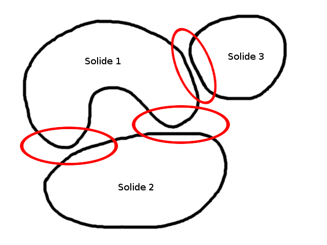
Figure 2.1-1: Definition of three contact areas
Case pairing MORTAR:
When we have calculations with incompatible meshes and we need to accurately estimate the contact states, we recommend using the MORTARLAC method. This calculation method makes it possible to make contact calculations on intersected couples SURFACE ESCL on SURFACE MAITcontrairement with the MAIT_ESCL pairing method which associates NOEUDSaux SEGMENTS.
To do this, there is a necessary step which is to pre-treat the mesh before using DEFI_CONTACT: CREA_MAILLAGE/DECOUPE_LAC. This step prepares the slave contact surface for integration of MORTAR contact terms on the intersected cells.
Because it uses a surface-surface approach, this method better respects the conditions of master/slave and slave/master interpenetrations. As with method MAIT_ESCL, the user must define potential contact areas couple by couple. There are no restrictions on the number of contact areas.
Two distinct areas may have common knots but no common stitches because the contact condition is imposed on the stitches. Moreover, within a zone, the master and slave surfaces of the same zone must also have a zero intersection. The kinematic contact quantities for method MORTAR are geometric fields per element.
2.2. Choice of master and slave surfaces#
As has just been said, each contact zone consists of a master surface and a slave surface. In the current state, you cannot do auto-contact in Code_Aster (except in the rare cases where you can predict the future contact zone and thus define a slave and a master).
The need to differentiate between the two surfaces comes from the technique adopted in calculating the game. This calculation is carried out in a phase called pairing.
In the case of pairing MAIT_ESCL, the game is defined at any point on the slave surface (for discrete methods these are nodes, for continuous methods integration points) as the minimum distance to the master surface. This asymmetry implies a choice that may*a priori* prove difficult (how to decide?). The points that should prevail in this choice are given in the following paragraphs.
In the case of pairing MORTAR, the game is defined by patching intersected slave-surface master.
These surfaces are entered in the operator DEFI_CONTACT under the keyword factor ZONE.
2.2.1. When a surface should be chosen as the master (GROUP_MA_MAIT)#
When one of these conditions is met:
one of the two surfaces is**rigid** (a);
one of the two surfaces**covers the other (b);
one of the two surfaces has an apparent stiffness**great** in front of the other (« apparent » in the sense that we are not talking about Young’s modules but about stiffness in \({\mathit{N.m}}^{\mathrm{-}1}\)) (c);
one of the two surfaces is meshed much more**coarse** than the other (d);
then this must be chosen as the master surface.
2.2.2. When a surface should be chosen as a slave (GROUP_MA_ESCL)#
When one of these conditions is met:
one of the two surfaces is**curve** (a);
one of the two surfaces is**smaller** than the other (b);
one of the two surfaces has an apparent stiffness**small** in front of the other (c);
one of the two surfaces is meshed much more**finely** than the other (d);
then this must be chosen as the slave surface.
2.2.3. General case#
When studying complex structures, the rules given in § 2.2.1 and § 2.2.2 may be difficult to apply. For example, when a solid is almost rigid (compared to the other solid) and is curved, rule (a) does not make it possible to decide: should one favor the curved character or the rigid character?
In these situations, the « art of the engineer » must prevail. In our example, if the two solids experience slight slips, the curved character of the rigid solid will have little influence and we will therefore choose the latter as the master surface.
When we encounter convergence problems (especially in plasticity), it is very likely that the choices on the master side slave are not wise. In this case change the role of surfaces.
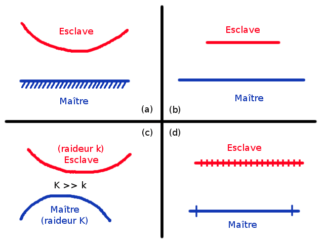
Figure 2.2.3-1: Choice of master and slave surfaces according to different situations
2.2.4. Orientation of the normals#
It is essential to always orient the normal contact surfaces so that they are outgoing. This can be done using the MODI_MAILLAGE operator. Depending on whether the surface to be oriented is a skin mesh of a massive element, a shell or a beam, the keywords ORIE_PEAU_2D or ORIE_PEAU_3D, ORIE_NORM_COQUE, ORIE_LIGNE will be used respectively.
In the case of ORIE_LIGNE, the tangent is oriented, so as to be able to systematically produce the normal by a vector product.
By default (keyword VERI_NORM of DEFI_CONTACT), the correct orientation of the normals is checked and the user is stopped if necessary.
2.2.5. Fineness and degree of meshing of curved surfaces#
When the contact surfaces are curved, it is necessary to guarantee the good continuity of the normal facets. To do this, we can either:
mesh finely linearly and use the smoothing option (cf. § 2.3.2)
mesh in quadratic
For the quadratic mesh to remain interesting, you must have placed the middle nodes on the geometry in the mesh and not have used the CREA_MAILLAGE/LINE_QUAD operator from Code_Aster.
Discreet Formulation Case:
In the case of quadratic contact surfaces, in discrete formulation, the contact surfaces should not be made up of quadrangular meshes with 8 knots (QUAD8) and we will therefore prefer 9-knot meshes (QUAD9) instead. We will then transform HEXA20 into HEXA27 and PENTA15 into PENTA18 (with the CREA_MAILLAGE operator). At present, mixed meshes that consist of both HEXA20 and PENTA15 cannot be transformed by CREA_MAILLAGE.
If, however, the use of HEXA20 elements is mandatory, the linear relationships written automatically on this occasion may be likely to conflict with boundary conditions (in particular symmetry), which is why it may be necessary to impose boundary conditions only on the vertex nodes of the QUAD8 cells concerned (one can use the DEFI_GROUP operator to create the ad-hoc group of nodes).
Continuous formulation case:
In continuous formulation (ALGO_CONT =” STANDARD “), for curved mesh sizes, the use of elements QUAD8ou **** TRIA6peut lead to violations of the law of contact**: the latter is verified on average. Slightly positive or slightly negative games are then observed in the presence of contact, which can disturb the results close to the contact zone or the calculations in recovery with the initial state. For this reason it is**advised** to use HEXA27 or PENTA18 elements (with QUAD9 faces) or linear elements.
When, at the end of a calculation, we notice a high rate of interpenetration of the master nodes inside the slave surfaces (which is possible, unlike the other way around), this generally means that the mesh of one or both surfaces is too coarse or that there is too great a difference in fineness between the two surface meshes. One can then either refine or invert master and slave.
If a surface is rigid (and therefore master), a coarse mesh is sufficient except of course in curved areas.
Finally, in the particular case of a cylinder-cylinder or sphere-sphere contact, care must be taken to mesh each surface sufficiently to avoid leaving too much void between them. In fact, in Code_Aster, we do not currently reposition nodes or projections on splines passing through the master surface, too coarse a mesh will then cause a strong oscillation in the contact pressure (detection of contact one node out of two).
In the case where there are oscillations in the contact pressures due to a highly incompatible mesh in the contact zone, the method ALGO_CONT =” LAC “ should be preferred.
2.2.7. Mesh quality#
The quality of the surface elements that constitute the master contact surface has a direct impact on the quality of the pairing. Indeed, distorted meshes, for example, can affect the precision of projections despite the robustness of the algorithm: the uniqueness of the projection is no longer guaranteed.
For these reasons, it is recommended to check the quality of the meshes produced and, if necessary, to correct their defects. In Code_Aster, the MACR_INFO_MAIL command allows you to display the distribution of elements according to their quality.
2.3. Pairing control#
2.3.1. Choosing the type of pairing#
In Code_Aster, three types of pairing are available:
« master-slave » (by default): it is the most generic, it prevents the nodes of the slave surface from penetrating the meshes of the master surface using orthogonal projections of a node on a mesh. It is available for discrete formulation and continuous formulation (** ALGO_CONT =” STANDARD “**).
« nodal »: it prevents slave nodes from entering master nodes in a direction (given by the normal slave). It is a pairing reserved for compatible meshes of contact surfaces for calculations in small slips. It is not available in continuous formulation (cf. § 3.1.3).
« MORTAR » (by default): it is the most qualitative, it makes it possible to impose the average contact conditions on the intersected meshes. With this method, interpenetration accuracies of less than 1.E -10% are achieved. It is available for continuous formulation only (** ALGO_CONT =” LAC “**).
2.3.2. Normals smoothing#
As the name suggests, this option allows you to smooth the normals. It is particularly useful in the case of curved surfaces meshed in linear fashion. This method is based on the average of the normals at the nodes, then their interpolation from the shape functions and the averaged normals, it ensures the continuity of the normal at the nodes.
The normal is then no longer the geometric normal, so we will take the precaution (recommended anyway) to check the results visually.
A verification of the facettization of the surfaces is carried out automatically at the end of the time step. It emits an information message when it becomes too important and it is then advisable to activate the smoothing.
2.3.3. Choice of normals: case formulation other than method LAC#
We recommend always leaving the default values: NORMALE =” MAIT “, VECT_MAIT =” AUTO”. That is, the non-penetration relationship is written from the master normal, determined using the mesh.
However, there are a few rare situations where you may want to impose the choice of normal: this is essentially the treatment of beam-beam contact (in 2D only) and the case where the master surface is a POI1 mesh. Refer to §3.1.6 of [U4.44.11] for more details.
2.3.4. Excluding slave nodes from pairing: case formulation other than method LAC#
The SANS_GROUP_NO/SANS_NOEUD keyword is used to exclude slave nodes from pairing. There may be several reasons for this:
master and slave surfaces have a non-empty intersection (crack bottom, rigid body movement blocking); common nodes do not need to be treated by contact, so they should be excluded.
linear relationships already exist on the slave nodes under consideration (boundary conditions, blocking rigid body movements); if these interfere with the direction of contact (respectively of friction), it is generally recommended to favor boundary conditions and therefore not to resolve the contact on these nodes.
A fatal error is issued when there are nodes that are common to master and slave surfaces and the master and slave surfaces have not been excluded.
2.4. Understanding geometric nonlinearity#
As explained, geometric nonlinearity results from the fact that it is necessary to apply frictional contact conditions to a geometric configuration that is not known. In this section, a short digression is made to explain the approach taken to overcome this difficulty.
2.4.1. Hypothesis of small slips#
The matching phase is a phase prior to the formulation of the contact conditions to be resolved. In practice, this means:
for discrete methods, the construction of a \(A\) matrix (for Matching) as multiplied by the displacement increment \(\delta u\) from the paired configuration, it gives the game increment (linearized).
for the continuous method, the association between a contact point and its projected into the parametric space of the paired master mesh. It is by updating the coordinates of the master mesh with the displacement \(\delta u\) that the new coordinates (linearized) of the projected are obtained.
Like the equilibrium conditions, the contact conditions are expressed on the deformed configuration (or final). This configuration is not known*a priori*.
The hypothesis of slight relative slips of the surfaces in contact is the analogue of the hypothesis of small disturbances (for writing equilibrium relationships).
It consists in saying that the final configuration of the surfaces in contact is little different from the initial configuration, which therefore makes it possible to perform the pairing once and for all at the beginning of the calculation on the initial configuration. Then use the conditions established on this configuration for all the calculation.
Such a problem is then linear geometrically: only the non-linearity of contact and friction remains, it is treated with adapted algorithms (cf. section 3).
2.4.2. General case#
To deal with problems of large relative slips of surfaces in contact, two possibilities exist: the use of a fixed point loop to reduce to cases of small slips or else for continuous formulation (§ 3.1.3) the simultaneous resolution within the Newton algorithm.
2.4.2.1. Fixed point loop (ALGO_RESO_GEOM =” POINT_FIXE “)#
The approach adopted is very similar to solving a non-linear problem using Newton’s method. We transform a geometric non-linear problem into a series of geometric linear problems. To do this, we will solve a series of problems in the hypothesis of small slips.
That is to say, we perform a pairing (on an initial balanced configuration) and a Newton resolution (with contact resolution as explained in section 3). This gives us a new configuration; if this configuration is « close » to the initial configuration then we have converged (so it was the final configuration), otherwise we loop: we do a pairing again then a resolution… and so on… and so on until we find the final configuration (cf.).
The difficulty is in characterizing the convergence of this fixed point process. What are two « close » configurations? In Code_Aster, these are two configurations whose « mechanical » displacement vector to go from one to the other (i.e. the displacement increment obtained by Newton restricted to the degrees of freedom DX, DY, DZ) has an infinite norm that is small compared to the infinite norm of the previous displacement vector.
This implies that we therefore always do at least two geometry iterations with this criterion (in order to give ourselves an initial displacement vector). Refer to paragraph 3.7 of [R5.03.50] for the exact expression of the infinite norm.
2.4.2.2. Generalized Newton algorithm (ALGO_RESO_GEOM =” NEWTON “)#
The continuous formulation (§ 3.1.3) offers the possibility of treating geometric nonlinearity directly within the Newton algorithm. To do this, a pairing is carried out at each iteration and the geometric terms of the tangent matrix are also updated.
The criterion of geometric convergence thus becomes an additional criterion of the Newton algorithm: the displacement increment must tend towards zero.
2.4.3. Convergence of the geometry loop#
2.4.3.1. Linearization of the normal#
The pairing provides two pieces of information:
the game on the paired configuration,
the coordinates of the potential contact point on the master surface.
Whether one uses a discrete or continuous contact method, one must derive (linearize) the principle of virtual powers, in particular the contact terms.
The fixed point hypothesis also leads to the assumption of a small variation in the normal during Newton iterations (of one step of time). This hypothesis is consistent with the small slippage hypothesis. The « game » operator is thus linearized more easily. In particular, it remains constant during a geometry iteration. This also has another implications: geometric convergence towards the final configuration in fixed point mode can sometimes be very slow.
Conversely, resolution by a generalized Newton method, possible only in continuous formulation (§ 3.1.3), presents a much faster convergence but may prove to be less robust. That’s why it’s not the default setting. To activate it, we will use the ALGO_RESO_GEOM keyword.
2.4.3.2. Geometric convergence criterion#
We saw above that the convergence of the geometry loop is based on a geometric criterion: the difference in the displacement vectors between two successive geometric configurations is relatively small. The displacement vectors are evaluated only on the contact zone. For the particular case of the generalized Newton algorithm in continuous formulation, the criterion applies directly to Newton’s displacement increment.
For fixed point loop resolution, « small » corresponds by default to less than 1% of the displacement since the start of the time step while with the generalized Newton algorithm, it is 0.0001% (this one benefiting from better convergence in favorable cases, in favorable cases, from better convergence, it is possible to require a tougher criterion).
When, as a result of a calculation, we observe an interpenetration of the slave nodes in the master surface, the only explanation [2] 2.2.5 is a non-verification of the geometric criterion.
You should then do not hesitate to harden the criterion. For this we use the keyword RESI_GEOM =0.005 in order to lower the threshold around 0.5% for example.
Sometimes geometric convergence is simply slow, in this case it is enough to increase the maximum number of iterations allowed: ITER_GEOM_MAXI =20 for example.
In some situations, no matter how much you play with the value of the criterion or the number of iterations, the calculation does not converge: it cycles. Several possibilities are then available to the user:
the most common explanation is a poor discretization of the contact surfaces (i.e. a too coarse mesh, a difference in fineness between the two surfaces or a poor choice of master and slave surfaces). We then refer to § 2.2.
when the contact surfaces are curved and meshed relatively roughly, the explanation may come from too great a discontinuity of the normal (facetting).**Activating smoothing then very often facilitates convergence**(cf. § 2.3.2). However, this should not prevent the user from reviewing their mesh.
if the case is really pathological, you have to force the number of updates yourself by using REAC_GEOM =” CONTROLE “and NB_ITER_GEOM =n. After \(n\) geometry iterations, the calculation will go to the next time step regardless of the value of the geometric criterion but it will emit an alarm when the criterion is not verified by less than 1% (for \(n\ge 2\)).
Figure 2.4.3.2-1: Treatment of the geometric nonlinearity of the contact by a fixed point loop
Note: In the case of the continuous formulation ALGO_CONT =” LAC “, there is no possibility to use ALGO_RESO_GEOM =” POINT_FIXE”.