3. Variational formulations#

Let’s transform the strong form of the problem into a weak formulation that is better suited to finite elements. Field \(u\) must belong to the \({V}_{0}\) set of kinematically eligible travel fields:

\({V}_{0}=\left\{v\in {H}^{1},v\text{discontinu}à\text{travers}{\Gamma }_{c},v=0\text{sur}{\Gamma }_{u}\right\}\)

3.1. Formulation for the regularized cohesive law#

We rate \(H\mathrm{=}{H}^{\mathrm{-}1\mathrm{/}2}(\Gamma )\) for cohesive laws. The weak formulation of the cohesive problem is written as follows:

Find \(\left(u,{t}_{c}^{\text{+}},{t}_{c}^{\text{-}}\right)\in {V}_{0}\times H\times H\) such as:

\({\int }_{\Omega }\sigma (u)\mathrm{:}\epsilon ({u}^{\text{*}})d\Omega ={\int }_{\Omega }f\cdot {u}^{\text{*}}d\Omega +{\int }_{{\Gamma }_{t}}t\cdot {u}^{\text{*}}\mathit{d\Gamma }+{\int }_{{\Gamma }^{\text{+}}}{t}_{c}^{\text{+}}\cdot {u}^{\text{*}\text{+}}{\mathit{d\Gamma }}^{\text{+}}+{\int }_{{\Gamma }^{\text{-}}}{t}_{c}^{\text{-}}\cdot {u}^{\text{*}\text{-}}{\mathit{d\Gamma }}^{\text{-}}\forall {u}^{\text{*}}\in {V}_{0}\)

Since \(⟦u⟧\left(x\right)={u}^{\text{+}}\left(x\right)-{u}^{\text{-}}\left(x\right)\) and \({t}_{c}={t}_{c}^{\text{-}}=-{t}_{c}^{\text{+}}\), the weak formulation is equivalently written as follows:

Find \(u\in {V}_{0}\) such as:

The current implementation actually includes a post-processing part, in order to give value to the unusual Lagrange multipliers:

Find \(\left(u,{\lambda }_{n},{\lambda }_{\tau }\right)\in {V}_{0}\times H\times H\) such as:

\(\forall \left({u}^{\text{*}},{\lambda }_{n}^{\text{*}},{\lambda }_{\tau }^{\text{*}}\right)\in {V}_{0}\times H\times H\)

Equation of balance	\(\begin{array}{c}{\int }_{\Omega }\sigma (u)\mathrm{:}\epsilon ({u}^{\text{}})d\Omega -{\int }_{\Omega }f\cdot {u}^{\text{}}d\Omega -{\int }_{{\Gamma }_{t}}t\cdot {u}^{\text{}}\mathit{d\Gamma }\\ +{\int }_{{\Gamma }_{c}}{t}_{c,n}\cdot {⟦{u}^{\text{}}⟧}_{n}{\mathit{d\Gamma }}_{c}+{\int }_{{\Gamma }_{c}}{t}_{c,\tau }\cdot {⟦{u}^{\text{*}}⟧}_{\tau }{\mathit{d\Gamma }}_{c}=0\end{array}\)
Post-treatment normal part	\({\int }_{\mathit{\Gamma c}}\left({\lambda }_{n}-{t}_{c,n}\cdot n\right){\lambda }_{n}^{\text{*}}{\mathit{d\Gamma }}_{c}=0\)
Tangential part post-treatment	\({\int }_{\mathit{\Gamma c}}\left({\lambda }_{\tau }-{t}_{c,\tau }\right){\lambda }_{\tau }^{\text{*}}{\mathit{d\Gamma }}_{c}=0\)

Thus, the multipliers \({\lambda }_{n}\) and \({\lambda }_{\tau }\) are not involved in the resolution. They are only used to store cohesive constraints explicitly.

3.2. Disadvantages of a cohesive regularized law#

In order to assess the ability of such a cohesive law to adequately describe the adherent zone, a test of openness of a circular inclusion is conducted. Geometry and loading are shown in figure (dimensions in millimeters). It is a plate under tension in plane deformations, with \(E=36.56\mathit{GPa}\) and \(\nu =0.2\). A circular inclusion is inserted into the plate, which is assumed to be able to open according to a cohesive law of critical stress \({\sigma }_{c}=2.7\mathit{MPa}\), and energetic toughness \({G}_{c}=0.095{\mathit{N.mm}}^{-1}\).

Figure 3.2-1: Test for the opening of a circular inclusion.

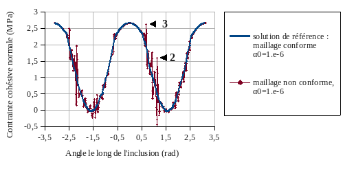
Figure 3.2-2: Normal cohesive force along the inclusion.

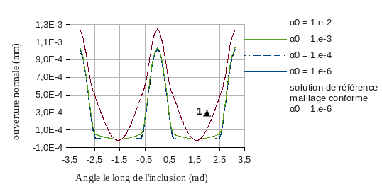
Figure 3.2-3: Normal movement jump along the inclusion.

The normal displacement jump and the force deduced therefrom are plotted in the figures and, for a loading \({u}_{0}=0.04\mathit{mm}\), for meshes that conform or do not conform to the cracked surface, and for penalty parameters \({\alpha }_{0}={10}^{-2}\) and \({\alpha }_{0}={10}^{-6}\). As we can see in the figures, regularized cohesive laws present three difficulties:

if the penalty is too low, the jump in movement along the inclusion is false: we observe an opening that is not physical (mark 1 in FIG.);
if, on the contrary, the penalty is too high, parasitic oscillations of the cohesive stress appear in the adherent zone (mark 2 in fig.). This problem has been reported extensively in the literature (see for example [bib3]). Originally noticed as part of the contact for Code_Aster, and referred to as « condition LBB », it is covered in the documentation [R5.03.54], §6. In short, it comes from the fact that the space for discretizing cohesive forces becomes too rich in comparison with that of displacement, when the stiffness of the law becomes such that one approaches a Dirichlet condition;
a poor evaluation of the operating system (adherent or dissipative) may occur as a result of these oscillations (mark 3 in the fig).

To conclude, penalized laws fail to give a faithful representation of adherent zones, since a penalty parameter \({\alpha }_{0}^{-1}\) that is too small implies a non-physical opening of the adherent zone, which leads to a false solution, while a parameter that is too large \({\alpha }_{0}^{-1}\) generates parasitic oscillations due to a stability problem, as soon as the penalization parameter begins to become sufficiently important to describe adherence appropriately.

By considering the pull-out test (this test is numerical, it does not correspond to any physical reality), it is possible to highlight the phenomenon of oscillations even more clearly.

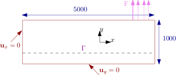
Figure 3.2-4: Pull-out test: geometry and loading.

The settings for this test are: \(E=30\mathit{GPa}\), \(\nu =0.2\),, \({\sigma }_{c}=0.2\mathit{MPa}\), \({G}_{c}=2\mathit{N.}{\mathit{mm}}^{-1}\), and \({\alpha }_{0}={10}^{-6}\). We have represented in figure the interface constraint for a conformal mesh, which is used as a reference, and the constraint for a non-conforming mesh. The phenomenon of parasitic oscillations of digital origin is particularly visible there throughout the adherent zone.

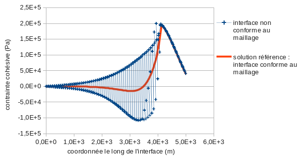
Figure 3.2-5: Pull-out test: cohesive stress along the interface.

3.3. Reduced space for discretizing the interface constraint#

For a detailed description of the discretization of contact unknowns, the reader can refer to the documentation [R5.03.54], §5. In short, the initial components of the multiplier are defined on the vertex nodes \(K\) of the intersected parent elements (see fig.). The implementation of such contact elements is detailed in [R5.03.54], §4. Equal relationships are then imposed between some of these initial components in order to result in a lower \({N}_{\lambda }\) number of degrees of liberty that are effectively independent. These relationships are supported by certain intersecting edges \(V\), called vital edges: a truly independent degree of freedom \(I\) is shared by a group of nodes of \(K\) (see fig.), which produces an extended contact form function \({\psi }_{I}\mathrm{:}=\sum _{i\in I}{N}_{i}\) (see fig.). The algorithm for selecting such vital edges, and therefore for constructing reduced space, is detailed in the documentation [R5.03.54], §6. The multiplier field is then obtained by interpolation on the parent elements and the discrete multiplier is the trace of this field on the interface:

math:: {M} _ {h}mathrm {:} =left{sum _ {I} {mu} _ {I} {psi} _ {I} {text {|}} {text {|}}} _ {text {|}}}} _ {Gamma}, {gamma}, {mu} _ {I} {I} {mu} _ {I} {d}right}}

Figure 3.3-1: Mesh not in accordance with the crack and reduced multiplier space.

3.4. Formulation for a mixed cohesive law for quadratic elements#

As opposed to the previous formulation, the treatment of such a law will require a real formulation with several fields, in the sense that a dual vector field \(\lambda\) will effectively enter the formulation, instead of being a post-processing device as in § 3.1. This formulation follows energetic reasoning, explained in detail in the documentation [R3.06.13]. Let’s summarize the main points:

We write that the opening of the crack costs an energy proportional to the area to be opened, that is:

\({E}_{\text{fr}}(\delta )\mathrm{=}\underset{\Gamma }{\mathrm{\int }}\Pi (\delta )\text{dS}\)

where \(\Pi (\delta )\) is the cohesive energy density. For law CZM_OUV_MIX, for example, we have \(\Pi (\delta )\mathrm{=}{\mathrm{\int }}_{0}^{{\delta }_{n}}{t}_{c,n}(\delta \text{'})d\delta \text{'}\).

The discontinuity field \(\delta\) appearing in the previous expressions is then defined as a field in its own right, integrated into the formulation as a new unknown. The total energy is then written as:

\(E(u,\delta )\mathrm{=}\underset{\Omega \mathrm{\setminus }\Gamma }{\mathrm{\int }}\Phi (\epsilon (u))d\Omega \mathrm{-}{W}_{\mathit{ext}}(u)+\underset{\Gamma }{\mathrm{\int }}\Pi (\delta )\mathit{d\Gamma }\)

The solution of the problem then consists in minimizing this total energy under the constraint that \(\delta\) corresponds to the displacement jump. We are looking for:

\(\underset{\begin{array}{c}u,\delta \\ \left[\left[u\right]\right]=\delta \end{array}}{\text{min}}E\left(u,\delta \right)\)

In order to solve this problem, we introduce the Lagrangian associated with the problem, to which we add an augmentation term whose usefulness will appear later:

\({L}_{r}\left(u,\delta ,\lambda \right)\underset{\mathit{déf.}}{=}E\left(u,\delta \right)+\underset{\Gamma }{\int }\lambda \cdot \left(⟦u⟧-\delta \right)\mathit{d\Gamma }+\underset{\Gamma }{\int }\frac{r}{2}{\left(⟦u⟧-\delta \right)}^{2}\mathit{d\Gamma }\)

We can then write the first optimality condition for this Lagrangian:

\(\forall {\delta }^{\text{*}}\underset{\Gamma }{\int }\left[{t}_{c}-\lambda +r\left(\delta -⟦u⟧\right)\right]\cdot {\delta }^{\text{*}}=0\text{avec}{t}_{c}\in \partial \Pi \left(\delta \right)\)

This equation involves the cohesive constraint \({t}_{c}\). However, we only have a local law of behavior as an expression of \({t}_{c}\). This first equation must therefore, in order to make sense, be discretized in a way that makes it possible to reduce it to a local expression. This is possible if \(\delta\) is discretized by collocation at the Gauss points of the interface, with coordinates \({x}_{g}\).

In fact, with such discretization, the resolution of the first optimum condition amounts to satisfying the cohesive law at each collocation point:

\({t}_{c}\left({\delta }_{g},{\alpha }_{g}\right)={\lambda }_{g}+r\left(⟦{u}_{g}⟧-{\delta }_{g}\right)\)

where we noted \({\lambda }_{g}\mathrm{=}\lambda ({x}_{g})\), for example, the values of a field at Gauss points, and where \({t}_{c}({\delta }_{g},{\alpha }_{g})\) follows the law. The graphical translation of this law of behavior is as follows: the solution corresponds to the intersection of the linear function \(\delta \to {\lambda }_{g}+r⟦{u}_{g}⟧-r\delta\) (with a negative slope given by the penalty coefficient \(r\)) with the graph \({t}_{c}(\delta ,\alpha )\). We then see that for \(r\) that is quite large, the solution is unique, which is why it is interesting to have increased the Lagrangian.

Figure 3.4-a: Behavioral integration solution.

Field \(\delta\) is therefore written locally as a function of \(\lambda +r⟦u⟧\), which we’ll call an increased multiplier and write it down as \(p\). As a result, unknown fields of the problem disappear. The formulation is then given by the two remaining Lagrangian optimality conditions:

Find \((u,\lambda )\mathrm{\in }{V}_{0}\mathrm{\times }H\) such as:

\(\mathrm{\forall }({u}^{\text{*}},{\lambda }^{\text{*}})\mathrm{\in }{V}_{0}\mathrm{\times }H\)

Equation of balance	\(\begin{array}{c}{\int }_{\Omega }\sigma (u)\mathrm{:}\epsilon ({u}^{\text{}})d\Omega -{\int }_{\Omega }f\cdot {u}^{\text{}}d\Omega -{\int }_{{\Gamma }_{t}}t\cdot {u}^{\text{}}d\Gamma \\ +{\int }_{{\Gamma }_{c}}\left[\lambda +r\left(⟦u⟧-\delta \left(p\right)\right)\right]\cdot ⟦{u}^{\text{}}⟧d\Gamma =0\text{avec}p=\lambda +r⟦u⟧\end{array}\)
Interface law	\({\int }_{{\Gamma }_{c}}\left[⟦u⟧-\delta (p)\right]\cdot {\lambda }^{\text{*}}d\Gamma =0\)

With regard to the discretization of these two fields of unknowns, a simple discretization respecting the condition of stability inf-sup, and consistent with the discretization of \(\delta\) by collocation, consists in discretizing the displacement with elements P 2 and the multiplier in a manner P 1 in a reduced space adapted to X- FEM, as detailed in § 3.3 or in [R5.03.54], §6.

3.5. Formulation for a mixed cohesive law for linear elements#

As demonstrated before, the quantities at the interface must be defined in a small space \({M}_{h}\) in order to prevent parasitic oscillations of numerical origin in the adherent phases. This applies to cohesive constraints \(\lambda\) and \({t}_{c}\). In fact, \({t}_{c}\) depends on \(\lambda +rw\) where \(w\) is the move jump. As a result of this increase, especially present during the adherent phases, \(w\) must also be written in the space consisting of \({M}_{h}\).

Note:

Another way to be convinced of this is to consider a problem of pure adherence, adherence being described by a regularized law. This problem in fact describes the behavior of the increase term during adherent phases. To avoid oscillations, we saw that a penalized law must be properly written on the reduced space, so the system to be solved is: \(\left[\begin{array}{ccc}{K}_{u}^{1}& 0& 0\\ 0& {K}_{u}^{2}& {A}^{T}\\ 0& A& \frac{1}{r}C\end{array}\right]\left\{\begin{array}{c}\{a\}\\ \{b\}\\ \{\lambda \}\end{array}\right\}=\left\{\begin{array}{c}\{{L}_{\text{méca}}^{1}\}\\ \{{L}_{\text{méca}}^{2}\}\\ 0\end{array}\right\}\)

where:

we group in \(\{{L}_{\text{méca}}\}\) and \([{K}_{u}]\) the discretization of all terms that are not interface terms;

:math:`{C}_{IK}={int }_{Gamma }{psi }_{I}{psi }_{K}dGamma`; *

:math:`{A}_{Ij}={int }_{Gamma }{psi }_{I}{varphi }_{j}dGamma`; *

*:math:`{a}`*is the vector combining the classic DDL movements; *

*:math:`{b}`*that of the enriched DDL; *

:math:`{lambda }`*groups DDL of the multiplier at the interface, discretization that takes place on the reduced space:math:`{M}_{h}`*; *

*:math:`r`*is the penalty setting. *

In a consistent penalized formulation, we can interpret the interface constraint as proportional to a consistent jump \(\{w\}\) : \(\{\lambda \}=r\{w\}\). With the previous matrix expression, we can then identify \(\{w\}={[C]}^{-1}[A]\{b\}\) .

We could then condense the previous matrix system to remove \(\{\lambda \}\) :

\([{K}_{u}^{2}]\{b\}+{[A]}^{T}\{\lambda \}=[{K}_{u}^{2}]\{b\}+{[A]}^{T}\left(r{[C]}^{-1}[A]\{b\}\right)\)

We then see that the resolution would require the assembly and calculation of a \({[A]}^{T}{[C]}^{-1}[A]\) matrix.

Such a matrix product is not feasible in an elementary calculation, all the more so given the non-local nature of \({M}_{h}\) . Such a global operation is therefore contrary to the computer architecture of Code_Aster, and should be prohibited as far as possible.

To overcome the problem, \(w\) is introduced as a new unknown to the problem, which is not discretized as \(⟦u⟧\) but is a projection onto a reduced space \({M}_{h}\). Decomposed using this field now available in the formulation, the previous stabilization term can be determined by assembling an elementary calculation. The total energy of the problem is written as:

\(E(u,\lambda ,w)=\frac{1}{2}{\int }_{\Omega }ϵ(u)\mathrm{:}C\mathrm{:}ϵ(u)d\Omega -{\int }_{{\Gamma }_{g}}g\cdot ud{\Gamma }_{g}+{\int }_{\Gamma }\Pi \left(w,\lambda \right)d\Gamma\)

The solution to the ongoing problem consists in minimization under the constraints of equality \(\left(u,w,\lambda \right)=\underset{{w}^{\text{*}}=⟦{u}^{\text{*}}⟧}{\mathit{argmin}}E\left({u}^{\text{*}},{\lambda }^{\text{*}},{w}^{\text{*}}\right)\). We can write the associated Lagrangian as:

\(L(u,w,\lambda ,\mu )=\frac{1}{2}{\int }_{\Omega }ϵ(u)\mathrm{:}C\mathrm{:}ϵ(u)d\Omega -{\int }_{{\Gamma }_{g}}g\cdot ud{\Gamma }_{g}+{\int }_{\Gamma }\Pi (w,\lambda )d\Gamma +{\int }_{\Gamma }\mu \cdot \left(⟦u⟧-w\right)d\Gamma\)

Writing the optimum conditions for this Lagrangian leads to the following variational formulation:

Equation of balance	\(\forall {u}^{\text{}}\in {V}_{h},{\int }_{\Omega }\sigma (u)\mathrm{:}ϵ({u}^{\text{}})d\Omega -{\int }_{{\Gamma }_{g}}g\cdot {u}^{\text{}}d{\Gamma }_{g}+{\int }_{\Gamma }\mu \cdot ⟦{u}^{\text{}}⟧d\Gamma =0\)
Move jump projection	\(\forall {\mu }^{\text{}}\in {M}_{h},{\int }_{\Gamma }\left(⟦u⟧-w\right)\cdot {\mu }^{\text{}}d\Gamma =0\)
Expression of cohesive force	\(\forall {w}^{\text{}}\in {M}_{h},-{\int }_{\Gamma }\left[\mu -{t}_{c}(\lambda +rw)\right]\cdot {w}^{\text{}}d\Gamma =0\)
Interface law	\(\forall {\lambda }^{\text{}}\in {M}_{h},-{\int }_{\Gamma }\frac{\left[\lambda -{t}_{c}(\lambda +rw)\right]}{r}\cdot {\lambda }^{\text{}}d\Gamma =0\)