2. Strong formulation of the cohesive problem#

2.1. Formulation of the equations of the general problem#

Note \(\Omega \subset {ℝ}^{d},d\in \{\mathrm{1,2}\}\) the uncracked calculation domain. Its border \(\mathrm{\partial }\Omega\) is divided into two parts \({\Gamma }_{u}\) and \({\Gamma }_{g}\), on which displacements and a density of surface forces \(t\) are respectively imposed (see fig.). We note \(\Gamma\) the potential crack zone on which the cohesive law is defined, composed of an upper crack lip \({\Gamma }^{\text{+}}\) and a lower lip \({\Gamma }^{\text{-}}\). If \({u}^{i}\) is the move on \({\Gamma }^{i}\), then we introduce the move jump as \(⟦u⟧\left(x\right)={u}^{\text{+}}\left(x\right)-{u}^{\text{-}}\left(x\right)\). Note \(n\) the normal vector coming out of \({\Gamma }^{\text{-}}\), \({n}^{\text{+}}\) the normal vector coming out of \({\Gamma }^{\text{+}}\), and \(-{t}_{c}^{\text{+}}={t}_{c}^{\text{-}}={t}_{c}\) the force [1] _ cohesive that applies to \({\Gamma }^{\text{-}}\) (see fig.). So on \(\Gamma\), we have \(-\sigma \cdot {n}^{\text{+}}=\sigma \cdot n={t}_{c}\). With these conventions, we have \(\mathrm{〚}{u}_{n}\mathrm{〛}\mathrm{=}\mathrm{〚}u\mathrm{〛}\mathrm{\cdot }n\) positive in openness and negative in interpenetration (see fig.).

Law of behavior	\(\sigma =C\mathrm{:}\epsilon \text{dans}\Omega\)
Balance	\(\nabla \cdot \sigma =f\text{dans}\Omega\)
Imposed surface forces	\(\sigma \cdot {n}_{\mathit{ext}}=t\text{sur}{\Gamma }_{t}\)
Density of cohesion efforts	\(\sigma \cdot n={t}_{c}\text{sur}\Gamma\)
Compulsory travel	\(u=0\text{sur}{\Gamma }_{u}\)

Table 2.1-1 : General problem equations.

Figure 2.1-1: Strong formulation of the cohesive problem.

2.2. Cohesive laws#

2.2.1. Regularized cohesive laws#

The first type of laws we can consider is a law in which the initial adherence is not perfect: the initial slope is finite. Two such cohesive laws are available in Code_Aster, laws CZM_EXP_REG and CZM_LIN_REG whose characteristics are detailed in [R7.02.11]. We recall the main points here, the reader can refer to them for more details. Here we detail the extension to XFEM for law CZM_EXP_REG, based on the reference article [bib 10]. The extension to law CZM_LIN_REG is made following exactly the same paradigm.

The opening of a crack in mixed mode is characterized by a damage criterion defined by means of the equivalent displacement jump and the internal variable \(\alpha\). The material remains in the elastic domain as long as the inequality is checked:

\(f({\mathrm{〚}u\mathrm{〛}}_{\mathit{eq}},\alpha )\mathrm{=}{\mathrm{〚}u\mathrm{〛}}_{\mathit{eq}}\mathrm{-}\alpha \mathrm{\le }0\)

\({⟦u⟧}_{\mathit{èq}}=\sqrt{{\langle ⟦{u}_{n}⟧\rangle }_{\text{+}}^{2}+{⟦{u}_{\tau }⟧}^{2}}\) is the equivalent movement jump,
\(\mathrm{〚}{u}_{\tau }\mathrm{〛}\mathrm{=}\mathrm{〚}u\mathrm{〛}\mathrm{-}\mathrm{〚}{u}_{n}\mathrm{〛}n\) is the tangential displacement jump,
\(\alpha (t)\mathrm{=}\mathit{max}\mathrm{\{}{\alpha }_{0},\underset{v\mathrm{\in }\mathrm{[}\mathrm{0,}t\mathrm{]}}{\mathit{max}}{\mathrm{〚}u(v)\mathrm{〛}}_{\mathit{éq}}\mathrm{\}}\) is the internal variable of the cohesive law,
\({\alpha }_{0}\) is the initial value for \(\alpha\). This value is given by the user via the material parameter PENA_ADHERENCE so that \({\alpha }_{0}\mathrm{=}\frac{{G}_{c}}{{\sigma }_{c}}\text{PENA\_ADHERENCE}\).

The cohesive stress is then written as the sum of an elastic stress, a dissipative stress and a penalization stress that takes into account the contact:

\({t}_{c}=H({〚u〛}_{\text{èq}}-\alpha ){\sigma }_{\mathrm{lin}}+(1-H({〚u〛}_{\text{èq}}-\alpha )){\sigma }_{\mathrm{dis}}+{\sigma }_{\mathrm{pen}}\)

where \(H\) is the indicator function of \({\mathrm{\Re }}^{+}\)

\({\sigma }_{\mathit{pen}}=C{\langle ⟦{u}_{n}⟧\rangle }_{\text{-}}n\) is the penalty requirement.

where \(C\) is a penalty coefficient explained in [R7.02.11] determined from the material parameter PENA_CONTACT.

\({\sigma }_{\mathit{lin}}={\sigma }_{\mathit{dis}}=\frac{{\sigma }_{c}}{\alpha }\mathrm{exp}(-\frac{{\sigma }_{c}}{{G}_{c}}\alpha )⟦u⟧\) is the expression common to linear and dissipative constraints, with \(\alpha \mathrm{=}{\mathrm{〚}u\mathrm{〛}}_{\mathit{èq}}\) for \({\sigma }_{\mathit{dis}}\).

where \({\sigma }_{c}\) is the critical stress at break and \({G}_{c}\) is the material’s energy toughness. In fact, it corresponds to the energy required for the complete opening of the interface over a unit length. A quick calculation using the preceding expressions confirms:

\(\underset{-\infty }{\overset{+\infty }{\int }}{t}_{c,\tau }\cdot d⟦{u}_{\tau }⟧+\underset{0}{\overset{+\infty }{\int }}\left({t}_{c}\cdot n\right)d⟦{u}_{n}⟧={G}_{c}\)

The figure shows the cohesive stress for a loading in pure \(I\) mode as a function of the normal displacement jump.

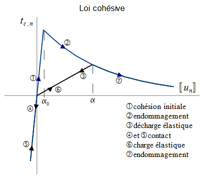
Figure 2.2.1-1 : Evolution of the normal cohesion force as a function of the displacement jump.

For \(\mathrm{〚}{u}_{n}\mathrm{〛}<0\), it is also usual to define an equivalent cohesive force \({t}_{c,\mathrm{eq}}\) using the equivalence energy condition:

\({t}_{c,\mathit{eq}}{\dot{⟦u⟧}}_{\mathit{eq}}={t}_{c,n}\dot{⟦{u}_{n}⟧}+{t}_{c,\tau }\cdot \dot{⟦{u}_{\tau }⟧}\)

To regain its value, we derive \({\mathrm{〚}u\mathrm{〛}}_{\mathit{èq}}\) with respect to time.

\(\dot{{\mathrm{〚}u\mathrm{〛}}_{\mathit{èq}}}\mathrm{=}\frac{\dot{\mathrm{〚}{u}_{n}\mathrm{〛}}\mathrm{〚}{u}_{n}\mathrm{〛}+\dot{\mathrm{〚}{u}_{\tau }\mathrm{〛}}\mathrm{\cdot }\mathrm{〚}{u}_{\tau }\mathrm{〛}}{{\mathrm{〚}u\mathrm{〛}}_{\mathit{èq}}}\)

Where do we identify: \({t}_{c,\mathit{èq}}={t}_{c,n}\frac{{⟦u⟧}_{\mathit{èq}}}{⟦{u}_{n}⟧}=\parallel {t}_{c,\tau }\parallel \frac{{⟦u⟧}_{\mathit{èq}}}{\parallel ⟦{u}_{\tau }⟧\parallel }=\frac{{\sigma }_{c}}{\alpha }\mathrm{exp}\left(-\frac{{\sigma }_{c}}{{G}_{c}}\alpha \right){⟦u⟧}_{\mathit{èq}}\)

The figure represents the evolution of the equivalent cohesion force as a function of the equivalent jump in displacement according to this law of behavior.

Figure 2.2.1-2 : Evolution of the equivalent cohesive force as a function of the equivalent jump in displacement.

Note:

\({t}_{c,\mathit{èq}}=\frac{{\sigma }_{c}}{\alpha }\mathrm{exp}\left(-\frac{{\sigma }_{c}}{{G}_{c}}\alpha \right){⟦u⟧}_{\mathit{èq}}\) An equivalent displacement jump is sometimes defined \({⟦u⟧}_{\mathit{èq}}=\sqrt{{\langle ⟦{u}_{n}⟧\rangle }_{\text{+}}^{2}+{\beta }^{2}{⟦{u}_{\tau }⟧}^{2}}\) where \(\beta\) is an experimental coefficient that represents the ratio of the intensity of the opening forces in mode \(I\) and in mode \(\mathit{II}\) . By then resuming the previous reasoning with: We deduce the expressions of the components:

\({t}_{c,n}=\frac{{t}_{c,\mathit{eq}}⟦{u}_{n}⟧}{{⟦u⟧}_{\mathit{èq}}}n=\frac{{\sigma }_{c}}{\alpha }\mathrm{exp}\left(-\frac{{\sigma }_{c}}{{G}_{c}}\alpha \right)⟦{u}_{n}⟧n\) , \({t}_{c,\tau }={\beta }^{2}\frac{{t}_{c,\mathit{eq}}⟦{u}_{\tau }⟧}{{⟦u⟧}_{\mathit{èq}}}={\beta }^{2}\frac{{\sigma }_{c}}{\alpha }\mathrm{exp}\left(-\frac{{\sigma }_{c}}{{G}_{c}}\alpha \right)⟦{u}_{\tau }⟧\)

2.2.2. Cohesive mixed laws for quadratic elements#

The second type of laws that we can consider is, conversely, a law in which the initial adherence is perfect: the initial slope is infinite. Two such cohesive laws are available with XFEM in Code_Aster, laws CZM_OUV_MIX and CZM_TAC_MIX whose characteristics are detailed in [R7.02.11]. Here we recall law CZM_OUV_MIX, shown in the figure.

By noting \(\delta\) the displacement jump (this is in order to comply with the notations of [R7.02.11]), the material remains in the elastic domain as long as:

\(f(\delta ,\alpha )={\delta }_{n}-\alpha \le 0\)

On the other hand, this time, the internal variable has an initial value that is strictly zero, so that the constraint is no longer explicit as a function of the displacement, as shown in the figure.

Figure 2.2.2-1: Normal component of the stress vector as a function of the normal jump for law CZM_OUV_MIX (threshold \(\alpha\) zero on the left and positive on the right).

2.2.3. Cohesive mixed laws for linear elements#

The law also has an infinite initial slope, but the discharge is linear (see fig.). It is available under vocabulary CZM_LIN_MIX. To lighten the ratings, let’s note \(w=⟦u⟧\). In the augmented Lagrangian formalism (see documentation [R5.03.52] and [R5.03.54]), a general expression for surface energy density is:

\(\Pi (w,\lambda )=\varphi (\lambda +rw)-\frac{\lambda \cdot \lambda }{2r}\)

where \(\varphi\) is a differentiable function, and \(r\) is an increase parameter.

The interface constraint is then classically given by a derivative with respect to the primal variable \({t}_{c}=\frac{\partial \Pi }{\partial w}\). An additional equation is needed to determine if one is in the adherent regime, and to impose the corresponding Dirichlet relationship if this is the case. In the augmented Lagrangian formalism, this additional interface law is determined by derivation with respect to the dual variable \(\frac{\partial \Pi }{\partial \lambda }=0\). The advantage of the augmented Lagrangian method is that there are no other inequalities to check during the resolution: the interface behavior is entirely contained in these two*equalities*, which allows the use of a Newton method for resolution.

The cohesive force is then:

\({t}_{c}\left(\lambda +rw\right)=\frac{\partial \Pi }{\partial w}=r\frac{\partial \varphi }{\partial (\lambda +rw)}\)

The interface law is then simply written as \(\frac{\partial \Pi }{\partial \lambda }=\frac{1}{r}\left[{t}_{c}\left(\lambda +rw\right)-\lambda \right]=0\), which can be rewritten \(\lambda ={t}_{c}\left(\lambda +rw\right)\) more simply.

Figure 2.2.3-1: Mixed cohesive law for linear elements.

An equivalent cohesive force is defined by \({\left(\lambda +rw\right)}_{\mathit{eq}}\mathrm{:}=\sqrt{{\langle {\lambda }_{n}+r{w}_{n}\rangle }_{\text{+}}^{2}+{\left({\lambda }_{\tau }+r{w}_{\tau }\right)}^{2}}\). A threshold function \(\phi\) is introduced by \(\phi \left({\left(\lambda +rw\right)}_{\mathit{eq}}\right)\mathrm{:}=\frac{{\left(\lambda +rw\right)}_{\mathit{eq}}-{\sigma }_{c}}{r{w}_{c}-{\sigma }_{c}}\). We can then define an internal variable adidimensional \(\alpha\) as the maximum of the threshold function over time, projected onto the \([\mathrm{0,1}]\) interval:

\(\stackrel{̃}{\alpha }(t)=\underset{[\mathrm{0,}t]}{\text{max}}\phi \left({\left(\lambda +rw\right)}_{\mathit{eq}}\right)\)

\(\alpha ={P}_{[\mathrm{0,1}]}(\stackrel{̃}{\alpha })\)

The value \(\alpha =0\) (or \(\stackrel{̃}{\alpha }\le 0\)) corresponds to a healthy material (adherent zone), and the value \(\alpha =1\) (or \(\stackrel{̃}{\alpha }\ge 1\)) corresponds to a completely cracked material (cracked zone). For load conditions, i.e. if \(\alpha =\phi \left({\left(\lambda +rw\right)}_{\mathit{eq}}\right)\), the function \(\varphi\) is defined by:

\(\varphi \left(\lambda +rw\right)=2{G}_{c}\left(1-\frac{{\sigma }_{c}}{r{w}_{c}}\right)\alpha \left(1-\frac{\alpha }{2}\right)+\frac{1}{2r}{\langle {\lambda }_{n}+r{w}_{n}\rangle }_{\text{-}}^{2}\)

An expression of the cohesive force \({t}_{c}=\frac{\partial \varphi }{\partial w}\) that derives from this energy can then be obtained. By defining an equivalent cohesive force as \({t}_{c,\mathit{eq}}=\sqrt{{\langle {t}_{c,n}\rangle }_{\text{+}}^{2}+{t}_{c,\tau }^{2}}\), the force/openness law can be expressed in terms of equivalent quantities like \({t}_{c,\mathit{eq}}=\left(1-{T}_{d}\right){\left(\lambda +rw\right)}_{\mathit{eq}}\), where \({T}_{d}\) is the damage function that corresponds to linear softening:

\({T}_{d}=\frac{\alpha }{\left(1-\frac{{\sigma }_{c}}{{w}_{c}r}\right)\alpha +\frac{{\sigma }_{c}}{{w}_{c}r}}\)

The vector relationship between cohesive force and displacement jump is then expressed in terms of normal component \({t}_{c,n}=\left(1-{T}_{d}\right){\langle {\lambda }_{n}+r{w}_{n}\rangle }_{\text{+}}+{\langle {\lambda }_{n}+r{w}_{n}\rangle }_{\text{-}}\) (the last term having been added to account for unilateral contact) and tangential component \({t}_{c,\tau }=\left(1-{T}_{d}\right)\left({\lambda }_{\tau }+r{w}_{\tau }\right)\).