3. Constitutive equations of the HM- XFEM model#
3.1. Equations for mechanics#
3.1.1. Equilibrium equation (case of the massif)#
In the case of the massif, the equation for the conservation of momentum (taking into account the volume forces) can be put in the form:
\(\text{Div}(\sigma )+r{F}^{m}=0\)
with:
\(\sigma ={\sigma }^{\text{'}}-\mathit{bp}1\) (under the assumption of effective constraints) where \(b\) is the Biot coefficient,
\(r\) the homogenized density such as in the saturated case \(r={r}_{0}+{m}_{w}\) where \({r}_{0}\) is the homogenized density in the reference configuration and \({m}_{w}\) the water mass inputs,
\(r{F}^{m}\) represent the volume forces acting on \(\Omega\) (in practice these are gravity forces).
3.1.2. Cohesive zone model (interface case)#
In order to take into account the propagation of the discontinuity, the irreversibility of the fracturing and the non-interpenetration of the lips of the discontinuity, we choose to model the behavior of the interface or the crack using a cohesive law.
For more information concerning the establishment of these laws, the user can refer to the documentation [R7.02.11]. As far as we are concerned, at the level of discontinuity, it is possible to distinguish 3 areas:
a completely open area, at which the total stress on the lips of the discontinuity is equal to \({p}_{f}{n}_{c}\) on \({\Gamma }_{2}\) and equal to \(-{p}_{f}{n}_{c}\) on \({\Gamma }_{1}\). In this zone the value of the stress is due mainly to the fluid flowing there,
a cohesive zone (or Fracture Processing Zone (FPZ)) whose opening depends on the value of the total stress which is then equal to \({t}_{c}={t}_{c}^{\text{'}}-{p}_{f}n\), \(n\) being the external normal to the surface concerned \({\Gamma }_{1}\) or \({\Gamma }_{2}\). Beyond a certain opening \({w}_{c}\), the constraint corresponds to that of the previous zone,
and a healthy adherent zone where the lips of the discontinuity are in contact and do not interpenetrate each other.
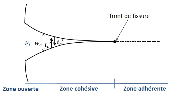
Figure 3.1.2-1: Distribution of stresses at the level of discontinuity On the are located the various stress zones associated with the cohesive zone model. The crack front is then naturally located at the border between the cohesive zone and the adherent zone.
The law of behavior used for cohesive laws takes the form of a softening relationship between the cohesive constraint \({t}_{c}\text{'}\) and the displacement jump \(⟦u⟧\) at the lips of the discontinuity.
Thus we pose:
\({t}_{c}\text{'}\phantom{\rule{0.5em}{0ex}}=\phantom{\rule{0.5em}{0ex}}\frac{\partial \mathrm{\psi }}{\partial ⟦u⟧}\)
with \(\psi\) the surface energy, whose expression depends on the cohesive law used.
The cohesive law adopted for hydromechanical XFEM elements is law CZM_LIN_MIX detailed in [R7.02.19]. It is a cohesive law that is not regularized (therefore with an infinite initial slope). \({\mathrm{\sigma }}_{c}\) is the critical stress at which damage starts in the cohesive zone. \({G}_{c}=\frac{{\mathrm{\sigma }}_{c}{w}_{c}}{2}\) corresponds to the quantity of energy to be supplied to completely break a unit of surface.
Figure 3.1.2-2: Mixed cohesive law.
3.1.3. Boundary conditions for mechanics#
Writing the boundary conditions for mechanics on the border of domain \(\Omega\) and at the interface level is written as:
Boundary conditions for mechanics |
|
3.2. Equations for hydrodynamics#
3.2.1. Mass conservation equation (case of the massif)#
In the case of the massif, the mass conservation equation takes the form:
\(\frac{\partial {m}_{w}}{\partial t}\text{}+\text{}\text{Div}(M)=0\)
with:
\({m}_{w}\) the mass inputs (per unit volume) expressed in \({\mathit{kg.m}}^{\text{-3}}\),
\(M\) the mass flows expressed in \({\mathit{kg.m}}^{\text{-2}}\mathrm{.}{s}^{\text{-1}}\).
3.2.2. Mass conservation equation (interface case)#
In the case of the interface, the mass conservation equation takes the form:
\(\frac{\partial w}{\partial t}\text{}+\text{}\text{Div}(W)=0\)
with:
\(w\) the mass contributions (per unit area) in the crack expressed in \({\mathit{kg.m}}^{\text{-2}}\),
\(W\) the mass fluxes in the crack expressed in \({\mathit{kg.m}}^{\text{-1}}\mathrm{.}{s}^{\text{-1}}\),
3.2.3. Boundary conditions for hydrodynamics#
Writing the boundary conditions for hydrodynamics on the border of domain \(\Omega\) and at the interface level makes it possible to obtain:
Boundary conditions for hydrodynamics |
|
An additional boundary condition to take into account is the continuity of the \({p}_{f}\) pressure at the level of each of the lips of the interface. This condition is necessary because of the very small thickness of the interface. It results in the following linear relationship:
\({p}^{\text{inf}}={p}_{f}\) out of \({\Gamma }_{1}\)
\({p}^{\text{sup}}={p}_{f}\) out of \({\Gamma }_{2}\)
with:
\({p}^{\text{sup}}\) the fluid pressure above the interface (field enriched by XFEM),
\({p}^{\text{inf}}\) the fluid pressure below the interface (field enriched by XFEM).
3.3. Equations of the poromechanical model#
In this part we are only recalling the useful equations of the poromechanical model developed in the documentation [R7.01.11].
3.3.1. Expression of mass inputs#
Case of the massif
Mass intakes can be put in the form (with \({S}_{\mathit{lq}}=1\)):
\({m}_{w}=\rho \varphi (1+{\epsilon }_{v})\)
with:
\(\rho ,\varphi\) respectively the density of water (in \({\mathit{kg.m}}^{\text{-3}}\)), the Eulerian porosity variable,
\({\epsilon }_{v}=\mathit{Tr}(\epsilon )=\mathit{Tr}({\nabla }_{s}u)\) volume deformation (where \(\mathit{Tr}\) is the linear trace application).
Interface case
Mass inputs can be in the form of:
\(w=\rho ⟦u⟧\mathrm{.}{n}_{c}\)
with:
\(\rho\) respectively the density of water,
\(⟦u⟧\mathrm{.}{n}_{c}\) the normal opening of the discontinuity (in \(m\)).
3.3.2. Expression of mass flows#
Case of the massif
The mass flow in the massif follows Darcy’s law. Thus we pose:
\(M=\lambda \rho (-\nabla p+\rho {F}^{m})\)
with \(\lambda =\frac{{K}^{\text{int}}}{{\mu }^{}}\) the mobility of the liquid where \({K}^{\text{int}}\) is the intrinsic permeability of the mass (in \({m}^{2}\)) and \(\mu\) the dynamic viscosity of the fluid (in \(\mathit{Pa.s}\)).
Note:
The expression of mobility actually involves the relative permeability of the fluid \({k}_{w}^{\text{rel}}({S}_{\text{w}})\) (which is a function of water saturation and is given by the law of Mualem/Van Genuchten [1 *0]) i.e.*i.e.* Given that the medium is saturated ( \({S}_{\text{w}}=1\) ), the relative permeability to water is therefore equal to \(1\):math:`lambda =frac{{K}^{text{int}}{k}_{w}^{text{rel}}}{{mu }^{}}` .
Interface case
The mass flow in the discontinuity can be written according to the cubic law [11] (we neglect the effects of gravity). Thus we pose:
\(W=-\frac{\rho {(⟦u⟧\mathrm{.}{n}_{c})}^{3}}{12\mu }\nabla {p}_{f}\)
with \(\mu\) the dynamic viscosity of the fluid (in \(\mathit{Pa.s}\)).
3.3.3. Evolution of the porosity variable#
The evolution of the porosity variable (Eulerian) characterizing the massif is given in the isothermal saturated case by:
\(d\varphi =(b-\varphi )\left(d{\epsilon }_{v}\text{}+\text{}\frac{\mathit{dp}}{{K}_{s}}\right)\)
with \({K}_{s}\) the compressibility module of the solid matrix (in \(\mathit{Pa}\)) and \(b\) the Biot coefficient.
3.3.4. Evolution of the density of the fluid#
Case of the massif
The evolution of the density of the fluid in the mass is given in the isothermal saturated case by:
\(\frac{d\rho }{{\rho }^{}}\text{}=\text{}\frac{\text{dp}}{{K}_{w}^{}}\)
with \({K}_{w}\) the coefficient of compressibility of the liquid (in \(\mathit{Pa}\)).
Interface case
The evolution of the density of the fluid at the interface level is given in the isothermal saturated case by:
\(\frac{d\rho }{{\rho }^{}}\text{}=\text{}\frac{{\text{dp}}_{f}}{{K}_{w}^{}}\)
3.3.5. Derived from mass inputs#
Since the differential of mass inputs is involved in the expression of the tangent operator associated with the linearized system (see § 6), its expression is recalled here in the case of saturated isothermal.
Case of the massif
First of all, the mass ratio differential can be written as:
\({\mathit{dm}}_{w}=\rho \varphi d{\epsilon }_{v}+\rho (1+{\epsilon }_{v})d\varphi +\varphi (1+{\epsilon }_{v})d\rho\)
Given the small disturbances hypothesis, for the sake of simplification, it is assumed that \((1+{\epsilon }_{v})\approx 1\). In the end (by replacing \(d\varphi\) and \(d\rho\) with their expressions):
\(d{m}_{w}=\rho bd{\epsilon }_{v}+\left(\left(\frac{\rho (b-\varphi )}{{K}_{s}^{}}+\frac{\rho \varphi }{{K}_{w}^{}}\right)\right)\mathit{dp}\)
Interface case
The difference in mass inputs is written as:
\(\mathit{dw}=\rho d(⟦u⟧\cdot {n}_{c})+(⟦u⟧\cdot {n}_{c})\rho \text{}\frac{d{p}_{f}}{{K}_{w}^{}}\)
3.3.6. Mass flow derivative#
Since the mass flow differential is involved in the expression of the tangent operator associated with the linearized system (see § 6) its expression is recalled here in the case of saturated isothermal.
Case of the massif
The mass flow differential in the case of the massif is written as:
\(dM=\left(\frac{M}{{\rho }^{\text{}}}+\rho \lambda {F}^{m}\right)\rho \text{}\frac{dp}{{K}_{w}^{}}+\frac{M}{{\lambda }^{\text{}}}d\lambda -\rho \lambda d\left(\nabla p\right)\)
Interface case
The mass flow differential in the case of the interface is written as:
\(dW\phantom{\rule{0.5em}{0ex}}=\phantom{\rule{0.5em}{0ex}}\left(\frac{W}{{\mathrm{\rho }}^{}}\right)\mathrm{\rho }\text{}\frac{dp}{{K}_{w}^{}}\phantom{\rule{0.5em}{0ex}}-\phantom{\rule{0.5em}{0ex}}\frac{\mathrm{\rho }}{12\mathrm{\mu }}\nabla {p}_{f}\left(3{\left(⟦u⟧\cdot {n}_{c}\right)}^{2}\right)d\left(⟦u⟧\cdot {n}_{c}\right)\phantom{\rule{0.5em}{0ex}}-\phantom{\rule{0.5em}{0ex}}\frac{\mathrm{\rho }{(⟦u⟧\cdot {n}_{c})}^{3}}{12\mathrm{\mu }}d\left(\nabla {p}_{f}\right)\)