5. Discretization of the problem#
5.1. Temporal discretization#
The equations for the conservation of mass in the case of the massif and the interface explicitly involve the time variable \(t\) in their formulations. In order to discretize these equations, we use a \(\theta\) -schema.
In terms of notation, a variable indexed by a \(\text{+}\) is a variable taken at the end of a time step and a variable indexed by a \(\text{-}\) is a variable taken at the beginning of a time step that is*a priori* known. We pose \(\Delta t\text{=}{t}^{\text{+}}-{t}^{\text{-}}\).
5.1.1. Discretization of the mechanical equation#
The time discretization of equations for mechanics does not involve a \(\theta\) -diagram. They are expressed at time \(\text{+}\text{}\) (i.e. after the prediction phase) and are written:
Equation of balance |
\(\forall {u}^{\text{*}}\in {U}_{\mathrm{0,}}{\int }_{\mathrm{\Omega }}{\mathrm{\sigma }}^{\text{+}}(u)\mathrm{:}\mathrm{ϵ}({u}^{\text{*}})d\mathrm{\Omega }-{\int }_{{\mathrm{\Gamma }}_{t}}{t}^{\text{+}}\cdot {u}^{\text{*}}d{\mathrm{\Gamma }}_{t}+{\int }_{{\mathrm{\Gamma }}_{c}}{\mathrm{\mu }}^{\text{+}}\cdot ⟦{u}^{\text{*}}⟧d{\mathrm{\Gamma }}_{c}=0\) |
Move jump projection |
\(\forall {\mathrm{\mu }}^{\text{*}}\in {L}_{0},{\int }_{{\mathrm{\Gamma }}_{c}}\left(⟦{u}^{\text{+}}⟧-{w}^{\text{+}}\right)\cdot {\mathrm{\mu }}^{\text{*}}d{\mathrm{\Gamma }}_{c}=0\) |
Expression of cohesive force |
\(\forall {w}^{\text{*}}\in {L}_{\mathrm{0,}}-{\int }_{{\mathrm{\Gamma }}_{c}}\left[{\mathrm{\mu }}^{\text{+}}-{t}_{c}^{\text{+}}({\mathrm{\lambda }}^{\text{+}}+r{w}^{\text{+}})\right]\cdot {w}^{\text{*}}d{\mathrm{\Gamma }}_{c}=0\) |
Interface law |
\(\forall {\mathrm{\lambda }}^{\text{*}}\in {L}_{\mathrm{0,}}-{\int }_{{\mathrm{\Gamma }}_{c}}\frac{\left[{\mathrm{\lambda }}^{\text{+}}-{t}_{c}^{\text{+}}({\mathrm{\lambda }}^{\text{+}}+r{w}^{\text{+}})\right]}{r}\cdot {\mathrm{\lambda }}^{\text{*}}d{\mathrm{\Gamma }}_{c}=0\) |
5.1.2. Discretization of hydrodynamic equations#
5.1.2.1. Case of the massif#
The time discretization of the mass conservation equation using a \(\theta\) -diagram is written:
\(\begin{array}{c}-{\int }_{\mathrm{\Omega }}\frac{{m}_{w}^{\text{+}}-{m}_{w}^{\text{-}}}{\mathrm{\Delta }t}{p}^{\text{*}}d\mathrm{\Omega }\text{}+\text{}\mathrm{\theta }{\int }_{\mathrm{\Omega }}{M}^{\text{+}}\cdot \nabla {p}^{\text{*}}d\mathrm{\Omega }\text{}+\text{}\left(1-\mathrm{\theta }\right){\int }_{\mathrm{\Omega }}{M}^{\text{-}}\cdot \nabla {p}^{\text{*}}d\mathrm{\Omega }\text{}\\ \text{=}\text{}\mathrm{\theta }{\int }_{{\mathrm{\Gamma }}_{F}}{M}_{\mathit{ext}}^{\text{+}}{p}^{\text{*}}d{\mathrm{\Gamma }}_{F}\text{}+\text{}\left(1-\mathrm{\theta }\right){\int }_{{\mathrm{\Gamma }}_{F}}{M}_{\mathit{ext}}^{\text{-}}{p}^{\text{*}}d{\mathrm{\Gamma }}_{F}\text{}-\text{}\mathrm{\theta }{\int }_{{\mathrm{\Gamma }}_{1}}{q}_{1}^{\text{+}}{p}^{\text{*}}d{\mathrm{\Gamma }}_{1}\\ \text{}-\text{}\left(1-\mathrm{\theta }\right){\int }_{{\mathrm{\Gamma }}_{1}}{q}_{1}^{\text{-}}{p}^{\text{*}}d{\mathrm{\Gamma }}_{1}\text{}-\text{}\mathrm{\theta }{\int }_{{\mathrm{\Gamma }}_{2}}{q}_{2}^{\text{+}}{p}^{\text{*}}d{\mathrm{\Gamma }}_{2}\text{}-\text{}\left(1-\mathrm{\theta }\right){\int }_{{\mathrm{\Gamma }}_{2}}{q}_{2}^{\text{-}}{p}^{\text{*}}d{\mathrm{\Gamma }}_{2}\hfill \end{array}\) \(\forall {p}^{\text{*}}\in {P}_{0}\)
5.1.2.2. Interface case#
The time discretization of the mass conservation equation using a \(\theta\) -diagram is written:
\(\begin{array}{c}-{\int }_{{\mathrm{\Gamma }}_{c}}\frac{{w}^{\text{+}}-{w}^{\text{-}}}{\mathrm{\Delta }t}{p}_{f}^{\text{*}}d{\mathrm{\Gamma }}_{c}\text{}+\text{}\mathrm{\theta }{\int }_{{\mathrm{\Gamma }}_{c}}{W}^{\text{+}}\cdot \nabla {p}_{f}^{\text{*}}d{\mathrm{\Gamma }}_{c}\text{}+\text{}\left(1-\mathrm{\theta }\right){\int }_{{\mathrm{\Gamma }}_{c}}{W}^{\text{-}}\cdot \nabla {p}_{f}^{\text{*}}d{\mathrm{\Gamma }}_{c}\text{}\\ \phantom{\rule{0.5em}{0ex}}=\phantom{\rule{0.5em}{0ex}}\mathrm{\theta }{\int }_{{\mathrm{\Gamma }}_{f}}{W}_{\mathit{ext}}^{\text{+}}{p}_{f}^{\text{*}}d{\mathrm{\Gamma }}_{f}\phantom{\rule{0.5em}{0ex}}+\phantom{\rule{0.5em}{0ex}}\left(1-\mathrm{\theta }\right){\int }_{{\mathrm{\Gamma }}_{f}}{W}_{\mathit{ext}}^{\text{-}}{p}_{f}^{\text{*}}d{\mathrm{\Gamma }}_{f}\phantom{\rule{0.5em}{0ex}}+\phantom{\rule{0.5em}{0ex}}\mathrm{\theta }{\int }_{{\mathrm{\Gamma }}_{1}}{q}_{1}^{\text{+}}{p}_{f}^{\text{*}}d{\mathrm{\Gamma }}_{1}\hfill \\ \text{+}\phantom{\rule{1em}{0ex}}\left(1-\mathrm{\theta }\right){\int }_{{\mathrm{\Gamma }}_{1}}{q}_{1}^{\text{-}}{p}_{f}^{\text{*}}d{\mathrm{\Gamma }}_{1}\phantom{\rule{0.5em}{0ex}}+\phantom{\rule{0.5em}{0ex}}\mathrm{\theta }{\int }_{{\mathrm{\Gamma }}_{2}}{q}_{2}^{\text{+}}{p}_{f}^{\text{*}}d{\mathrm{\Gamma }}_{2}\hfill \\ \phantom{\rule{0.5em}{0ex}}+\phantom{\rule{0.5em}{0ex}}\left(1-\mathrm{\theta }\right){\int }_{{\mathrm{\Gamma }}_{2}}{q}_{2}^{\text{-}}{p}_{f}^{\text{*}}d{\mathrm{\Gamma }}_{2}\hfill \end{array}\) \(\forall {p}_{f}^{\text{*}}\in {F}_{0}\)
5.1.3. Discretization of the equations of the poromechanical model#
The equations presented in this part correspond to the equations in § 3.3 expressed incrementally. We develop these equations because they are affected by discretization with XFEM.
5.1.3.1. Case of mass inputs#
Case of the massif
The mass inputs are then written incrementally:
\({m}_{w}^{\text{+}}-{m}_{w}^{\text{-}}={\rho }^{\text{+}}{\varphi }^{\text{+}}\left(1+{\epsilon }_{v}^{\text{+}}\right)-{\rho }^{\text{-}}{\varphi }^{\text{-}}\left(1+{\epsilon }_{v}^{\text{-}}\right)\)
Interface case
The mass inputs are then written incrementally:
\({w}^{\text{+}}-{w}^{\text{-}}={\rho }^{\text{+}}{\left(⟦u⟧\cdot {n}_{c}\right)}^{\text{+}}-{\rho }^{\text{-}}{\left(⟦u⟧\cdot {n}_{c}\right)}^{\text{-}}\)
5.2. Discretization with XFEM#
5.2.1. Representation of the element HM- XFEM and associated ddls#
To represent the HM- XFEM element, we chose to use quadratic elements that can be either quadrangles with 8 knots (QUAD8) or triangles with 6 knots (TRIA6), or hexahedra with 20 knots (HEXA20), or pentahedra with 15 knots (PENTA15), or pentahedra with 15 knots (), or pyramids with 13 knots (PYRA13), or tetrahedra with 10 knots (), or pentahedra with 15 knots (), or pyramids with 13 knots (). TETRA10). We consider that any element of the mesh crossed by the interface is of the type HM- XFEM. This element is surrounded by non-enriched HM elements. These are the ones used classically for HM models.
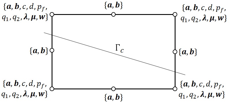
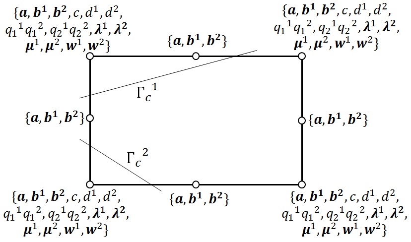
The figure shows the element HM- XFEM with a QUAD8 mesh.
|
Figure 5.2.1-1: Representation of the element HM- XFEM with QUAD8
In each of the figures presented above, the lists at each node of the element contain the degrees of freedom (ddls) associated with each node category (vertex nodes or middle nodes).
Degrees of freedom:
\(a\) and \(b\) are respectively associated with the classical and enriched part of the approximation of the travel field \({u}^{h}\),
\(c\) and \(d\) are respectively associated with the classical and enriched part of the approximation of the pressure field in massif \({p}^{h}\),
\({p}_{f}\) are associated with the approximation of the \({p}_{f}^{h}\) pressure field at the interface level,
\({q}_{1}\) and \({q}_{2}\) are associated with the approximation of the hydraulic Lagrange multiplier fields \({q}_{1}^{h}\) and \({q}_{2}^{h}\).
\(\mathrm{\lambda }\), \(\mathrm{\mu }\) and \(w\) are respectively associated with the approximation of the Lagrange multipliers \({\mathrm{\lambda }}^{h}\) and \({\mathrm{\mu }}^{h}\) and the displacement jump \({w}^{h}\).
The hydromechanical elements present in Code_Aster use « mixed interpolation », in order to reduce the oscillations of the numerical solution [14]. The displacement field is thus interpolated quadratically while the pore pressure field is interpolated linearly. The degrees of freedom \(c\) and \(d\) are therefore only carried by the vertex nodes while the degrees of freedom \(a\) and \(b\) are carried by both the middle nodes and the vertex nodes. With regard to the fields associated with discontinuities: \({p}_{f}^{h}\), \({q}_{1}^{h}\), \({q}_{2}^{h}\),,,, \({\mathrm{\lambda }}^{h}\), \({\mathrm{\mu }}^{h}\) and \({w}^{h}\), the degrees of freedom are carried only by the vertex nodes. In addition, their approximation space is reduced (see § 5.2.2) in order to respect the stability condition LBB [8,9]. This condition in fact imposes a hierarchy between the approximation spaces, without which we observe the appearance of oscillations and the non-uniqueness of the solution of the coupled problem.
In addition, it is important to note that HM- XFEM elements that share vertex nodes with conventional HM elements must undergo additional processing. It is in fact necessary to zero the enriched degrees of freedom (for the fields of pressure in the mountains and for movements) but also to zero the degrees of freedom \({p}_{f}\), \({q}_{1}\), \({q}_{2}\), \(\mathrm{\lambda }\), \(\mathrm{\mu }\) and \(w\) at the level of the summit nodes in common between these two types of element. The disposal procedure used is that described in § 4.4 of the [R5.03.54] documentation.
Here we summarize the problem points associated with the cohabitation between the HM- XFEM elements and the classical HM elements.
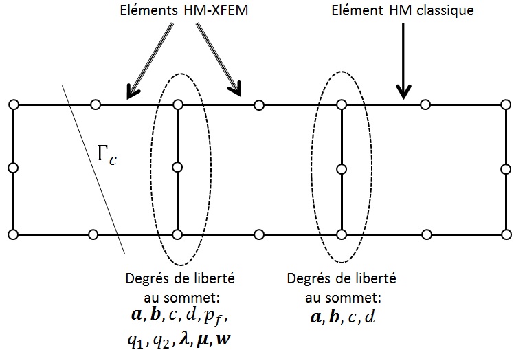
Figure 5.2.1-1: Cohabitation of the HM- XFEM element with the classical HM element
5.2.2. Reduced space for discretizing fields associated with discontinuity#
For a detailed description of the discretization of contact unknowns (and a fortiori of all the unknowns associated with discontinuity), the reader can refer to the documentation [R5.03.54], §5. In short, the initial components of the multiplier are defined on the vertex nodes \(K\) of the intersected parent elements (see fig.). The implementation of such contact elements is detailed in [R5.03.54], §4. Equal relationships are then imposed between some of these initial components in order to achieve a lower number \({N}_{\mathrm{\lambda }}\) of effectively independent degrees of freedom. These relationships are supported by certain intersecting edges \(V\), called vital edges: a truly independent \(I\) degree of freedom is shared by a group of nodes of \(K\) (see fig.), which produces an extended contact form function \({\mathrm{\psi }}_{I}\mathrm{:}=\sum _{i\in I}{N}_{i}\) (see fig.). The algorithm for selecting such vital edges, and therefore for constructing reduced space, is detailed in the documentation [R5.03.54], §6. The multiplier field is then obtained by interpolation on the parent elements and the discrete multiplier is the trace of this field on the interface:
- math:
{M} _ {h}mathrm {:} =left{sum _ {I} {mathrm {mu}} _ {I} {mathrm {psi}} _ {I} {psi}}} _ {I} {text {:}} =left{text {|}} =left{text {|}} =left{sum_ {I} {psi}} _ {I} {psi}}} _ {I} {psi}} _ {I} {psi}} _ {I} {psi}} _ {I} {psi}} _ {I} {psi}}} _ {I} {psi}} _ {I} {psi}}} _ {I} thrm {328}} ^ {d}right}
Figure 5.2.2-1: Mesh not in accordance with the crack and reduced space for the interface
In our case, the fields associated with the discontinuity are not only the Lagrange multipliers \(\mathrm{\lambda },\mathrm{\mu }\) and the displacement jump \(w\) useful for the cohesive law CZM_LIN_MIXmais also the hydraulic fields associated with the discontinuity: the fluid pressure in the discontinuity \({p}_{f}\), and the flows \({q}_{1}\) and \({q}_{2}\). These fields are all discretized on the reduced space \({M}_{h}\).
5.2.3. Field approximations with XFEM#
The approximation of the fields present can therefore be put in the form (the test fields used in the weak forms of the equilibrium equations are approximated in the same way):
for the travel field:
\({u}^{h}(x)=\sum _{i=1}^{\mathit{nn}}{a}_{i}{\mathrm{\phi }}_{i}(x)\phantom{\rule{0.5em}{0ex}}+\phantom{\rule{0.5em}{0ex}}\sum _{j=1}^{\mathit{nne}}{b}_{j}{\mathrm{\phi }}_{j}(x)\stackrel{~}{H}(\mathit{lsn}(x))\)
for the pressure field in the massif:
\({p}^{h}(x)=\sum _{i=1}^{\mathit{nns}}{c}_{i}{\mathrm{\psi }}_{i}(x)\phantom{\rule{0.5em}{0ex}}+\phantom{\rule{0.5em}{0ex}}\sum _{j=1}^{\mathit{nnse}}{d}_{j}{\mathrm{\psi }}_{j}(x)\stackrel{~}{H}(\mathit{lsn}(x))\)
for the pressure field in the interface:
\({p}_{f}^{h}(x)=\sum _{i=1}^{\mathit{nnc}}{({p}_{f})}_{i}\stackrel{~}{{\mathrm{\psi }}_{i}}(x)\)
for hydraulic Lagrange multiplier fields:
\({q}_{1}^{h}(x)=\sum _{i=1}^{\mathit{nnc}}{({q}_{1})}_{i}\stackrel{~}{{\mathrm{\psi }}_{i}}(x)\)
\({q}_{2}^{h}(x)=\sum _{i=1}^{\mathit{nnc}}{({q}_{2})}_{i}\stackrel{~}{{\mathrm{\psi }}_{i}}(x)\)
for the Lagrange multiplier fields and the displacement jump useful for the cohesive zone model:
\({\mathrm{\lambda }}^{h}(x)=\sum _{i=1}^{\mathit{nnc}}{\mathrm{\lambda }}_{i}\stackrel{~}{{\mathrm{\psi }}_{i}}(x)\)
\({\mathrm{\mu }}^{h}(x)=\sum _{i=1}^{\mathit{nnc}}{\mathrm{\mu }}_{i}\stackrel{~}{{\mathrm{\psi }}_{i}}(x)\)
\({w}^{h}(x)=\sum _{i=1}^{\mathit{nnc}}{w}_{i}\stackrel{~}{{\mathrm{\psi }}_{i}}(x)\)
with:
:math:`mathit{lsn}` the normal*level set*whose iso-zero represents the interface. For more details on the use of*level set*with XFEM in*Code_Aster, the reader can refer to the documentation [R7.02.13],
\(\stackrel{~}{H}\) the discontinuous function through the discontinuity identified by \(\mathit{lsn}(x)=0\) (confer [R7.02.12])
\({\phi }_{i}(x)\) the quadratic element shape functions used for the interpolation of the displacement field,
\({\psi }_{i}(x)\) the shape functions of the linear parent element used for the interpolation of the pressure field in the massif.
\(\stackrel{~}{{\mathrm{\psi }}_{i}}(x)\) the linear form functions used for the interpolation of fields associated with discontinuity. They differ from the shape functions of the linear parent element \({\psi }_{i}(x)\) in the case where vertex nodes of the linear parent element do not belong to any edge intersected by the discontinuity (see § 5.4 and [R5.03.54] for more details). This situation only occurs for non-simplistic elements.
\(\mathit{nn}\) the set of mesh nodes and \(\mathit{nne}\) the set of enriched mesh nodes.
\(\mathit{nn}\) the set of vertex nodes in the mesh and \(\mathit{nne}\) the set of enriched vertex nodes in the mesh.
\(\mathit{nnc}\) the vertex nodes belonging to an edge intersected by the \({\mathrm{\Gamma }}_{c}\) discontinuity.
Note:
As we can see in defining the approximations of the displacement and pressure fields of the massif, the enrichment due to the presence of a crack point is not taken into account. In the formulation of the mechanical problem, we are based on a model of regulated cohesive zones. The advantage of such a model (historically introduced by Barenblatt [12] in order to improve Griffith’s theory concerning fractured environments [13]) is to overcome the fact that the stresses are infinite at the crack point. Therefore, the enrichment of the displacement field approximation by singular functions is inappropriate here, but entirely feasible with respect to the enrichment of the pressure field approximation in the massif as suggested by [7].
5.3. Extension to the multi-cracked case#
5.3.1. Representation of the multi-cracked element HM- XFEM and associated ddls#
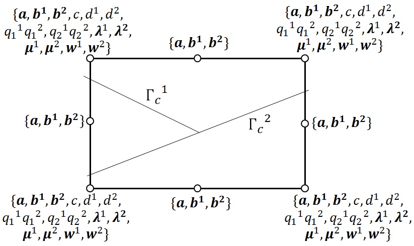
In Code_Aster, XFEM elements can support up to 4 cracks per element (see [R7.02.12]). It is also possible to have connected cracks. In particular, these features are available for HM- XFEM elements. To each additional crack, a set of degrees of freedom enriched for the field of displacement and pore pressure as well as a set of degrees of freedom associated with the additional discontinuity is added. In the Figure, we represent an HM- XFEM QUAD8 element intersected by two interfaces (not connected to the left and connected to the right) as well as the degrees of freedom carried by each of the nodes.
|
|
Figure 5.3.1-1: Representation of an HM- XFEM QUAD8 element intersected by two discontinuities that are not connected (on the left) and connected (on the right)
5.3.2. Field approximations with XFEM in the multi-cracked case#
In the case where several cracks intersect the same mesh, for each node, a correspondence is established between each interface and the enriched degrees of freedom and interface (see [R7.02.12]). Thus, the approximation of the fields present can be put in the following form:
for the travel field:
\({u}^{h}(x)=\sum _{i=1}^{\mathit{nn}}{a}_{i}{\mathrm{\phi }}_{i}(x)\phantom{\rule{0.5em}{0ex}}+\phantom{\rule{0.5em}{0ex}}\sum _{\mathit{ifiss}=1}^{\mathit{nfiss}}\sum _{j=1}^{\mathit{nne}}{b}_{j}^{\mathrm{\alpha }(\mathit{ifiss},j)}{\mathrm{\phi }}_{j}(x)\stackrel{~}{H}({\mathit{lsn}}_{\mathit{ifiss}}(x))\)
for the pressure field in the massif:
\({p}^{h}(x)=\sum _{i=1}^{\mathit{nns}}{c}_{i}{\mathrm{\psi }}_{i}(x)\phantom{\rule{0.5em}{0ex}}+\phantom{\rule{0.5em}{0ex}}\sum _{\mathit{ifiss}}^{\mathit{nfiss}}\sum _{j=1}^{\mathit{nnse}}{d}_{j}^{\mathrm{\alpha }(\mathit{ifiss},j)}{\mathrm{\psi }}_{j}(x)\stackrel{~}{H}({\mathit{lsn}}_{\mathit{ifiss}}(x))\)
for interface degrees of freedom, for example, for fluid pressure \({p}_{f}\) in interface \(\mathit{ifiss}\), we have:
\({p}_{f}^{h,\mathit{ifiss}}(x)=\sum _{i=1}^{\mathit{nnc}}{({p}_{f}^{\mathrm{\alpha }(\mathit{ifiss},i)})}_{i}\stackrel{~}{{\mathrm{\psi }}_{i}}(x)\)
with:
\(\mathrm{\alpha }\) the function that associates with each interface the enriched degree of freedom or associated interface number for each node.
5.3.3. Hydraulic fracture junction#
The fields associated with each interface are therefore discretized with distinct sets of degrees of freedom. The interfaces therefore function independently, even if they exert their influence on each other via the porous matrix. In the case of a hydraulic interface junction, it is however appropriate to impose a hydraulic connection, in order to allow fluid exchanges at the junction (see Figure). To this end, we can either impose the conservation of mass at the junction (law of nodes on flows \(W\) in each branch of the junction), or impose the continuity of pressure \({p}_{f}\) in the cracks at the junction.
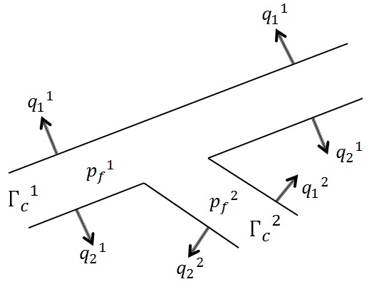
Figure 5.3.3-1: Hydraulic crack junction
Given the limited approximation space we have for field \({p}_{f}\), it is preferable to impose the continuity of the \({p}_{f}\) pressure at the junction, rather than to impose an equality on the flows \(W\) that involve the gradient of \({p}_{f}\). To this end, a node carrying the degree of freedom \({p}_{f}\) is identified for both the main crack and the branched crack and the equality of these two degrees of freedom is imposed (see Figure).
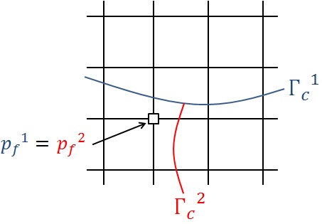
Figure 5.3.3-2: Imposition of the continuity of pressure \({p}_{f}\) in hydraulic cracks at a junction.
5.4. Imposition of a flow in a hydraulic interface#
With regard to the surface fluid flows injected into the porous matrix, the integration of the second member occurs naturally on the edge \({\mathrm{\Gamma }}_{F}\) on which the flow \({M}_{\mathit{ext}}\) is imposed (see § 4.2.1), of dimension \(\mathit{ndim}-1\) if the dimension of the domain \(\mathrm{\Omega }\) is \(\mathit{ndim}\). On the other hand, when it comes to imposing a flow of fluid directly into the fracture, the dimension of the mouth \({\mathrm{\Gamma }}_{f}\) is \(\mathit{ndim}-2\) if the dimension of the domain \(\mathrm{\Omega }\) is \(\mathit{ndim}\). The integration of feed flow \({W}_{\mathit{ext}}\) therefore requires more attention. First, let’s look at the case where the dimension of \(\mathrm{\Omega }\) is \(2\). The \({W}_{\mathit{ext}}\) flow is then expressed in \(\mathit{kg}\mathrm{.}{s}^{-1}\) and \({\mathrm{\Gamma }}_{f}\) is reduced to one point. Recall that the approximation space for fields associated with the cohesive interface like \({p}_{f}\) is based only on the node vertices of the edges strictly intersected by the interface and on the nodes over which the interface passes. In the Figure, the nodes that actually carry the degree of freedom \({p}_{f}\) are marked by white and red squares. The integration of the term \({\int }_{{\mathrm{\Gamma }}_{f}}{W}_{\mathit{ext}}{p}_{f}^{\text{*}}d{\mathrm{\Gamma }}_{f}\) will therefore be based on the restriction of this approximation space at the edge of the domain. In the case where the cohesive interface is consistent with the edge of the domain, \({W}_{\mathit{ext}}\) will be directly imposed on the \({N}_{1}\) node (see right). In the non-compliant case, we will have to determine the relative distance \(\mathrm{\alpha }\) between the mouth \(I\) and the summit nodes of the intersected edge \({N}_{1}\) and \({N}_{2}\) (see left). We will then impose \((1-\mathrm{\alpha }){W}_{\mathit{ext}}\) on the \({N}_{1}\) node and \(\mathrm{\alpha }{W}_{\mathit{ext}}\) on the \({N}_{2}\) node.
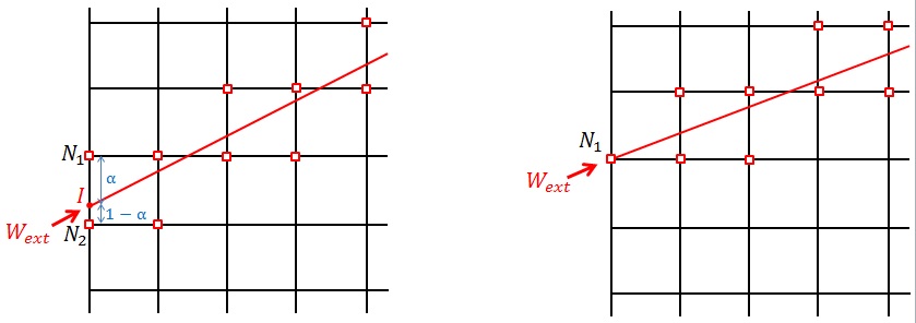
Figure 5.4-1: Imposition of a flow in a fracture for 2D plane models in the non-compliant case (left) and in the compliant case (right).
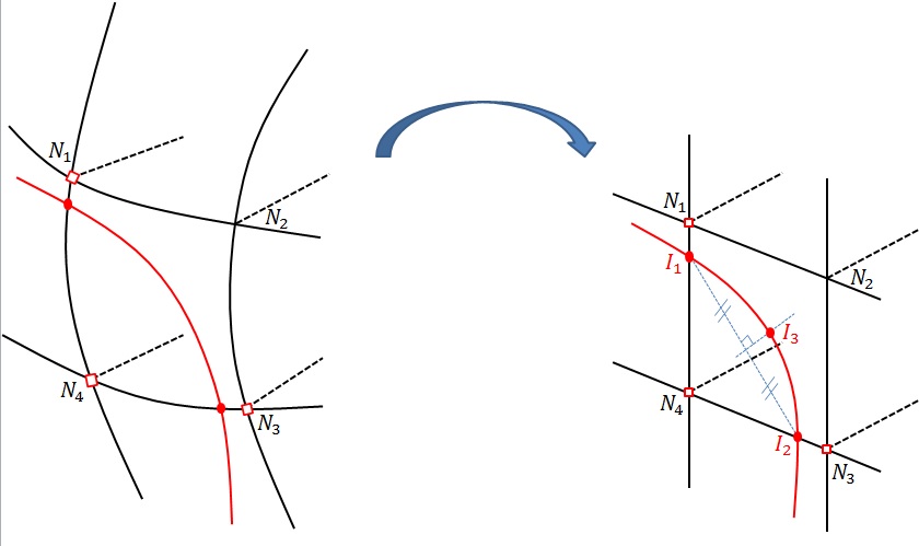
In the case where the dimension of \(\mathrm{\Omega }\) is \(3\), the flow \({W}_{\mathit{ext}}\) is expressed in \(\mathit{kg}\mathrm{.}{m}^{-1}\mathrm{.}{s}^{-1}\) and \({\mathrm{\Gamma }}_{f}\) is a curve. In order to integrate the term \({\int }_{{\mathrm{\Gamma }}_{f}}{W}_{\mathit{ext}}{p}_{f}^{\text{*}}d{\mathrm{\Gamma }}_{f}\), it is necessary to have a support that approximates the \({\mathrm{\Gamma }}_{f}\) curve. To this end, we reconstruct an approximation of the interface on the edge of the domain as a chain of segments with 3 nodes. In each edge face, interface \({\mathrm{\Gamma }}_{c}\) is discretized by a segment with 3 nodes. To do this, we use the same procedure as for creating integration sub-elements XFEM (see [R7.02.12]). The edge faces intersected by \({\mathrm{\Gamma }}_{c}\) are flipped into the reference space (see). We then determine the intersections \({I}_{1}\) and \({I}_{2}\) with the edges of the face that will constitute the end nodes of the 3-node segment. Then we determine the position of the middle node \({I}_{3}\) on the mediator of the segment \([{I}_{1}{I}_{2}]\). A quadratic approximation of the interface at the edge of domain \(\mathrm{\Omega }\) is then obtained. We are then in a position to evaluate \({\int }_{{\mathrm{\Gamma }}_{f}}{W}_{\mathit{ext}}{p}_{f}^{\text{*}}d{\mathrm{\Gamma }}_{f}\) by integrating 3-node segments into the chain that approximate \({\mathrm{\Gamma }}_{f}\). However, you must be careful with the approximation space of \({p}_{f}\) on the intersected faces. As mentioned earlier, the approximation space for field \({p}_{f}\) is based only on the node vertices of the edges strictly intersected by the discontinuity and the nodes over which the discontinuity passes. In the Figure, only nodes \({N}_{1}\), \({N}_{3}\), and \({N}_{4}\) on the quadrangle edge face have the degree of freedom \({p}_{f}\). In order to still satisfy the partition of the unit in the quadrangle face, modified form functions are used for field \({p}_{f}\):
\(\begin{array}{c}\stackrel{~}{{\mathrm{\psi }}_{{N}_{1}}}={\mathrm{\psi }}_{{N}_{1}}+\frac{{\mathrm{\psi }}_{{N}_{2}}}{3}\\ \stackrel{~}{{\mathrm{\psi }}_{{N}_{2}}}=0\\ \stackrel{~}{{\mathrm{\psi }}_{{N}_{3}}}={\mathrm{\psi }}_{{N}_{3}}+\frac{{\mathrm{\psi }}_{{N}_{2}}}{3}\\ \stackrel{~}{{\mathrm{\psi }}_{{N}_{4}}}={\mathrm{\psi }}_{{N}_{4}}+\frac{{\mathrm{\psi }}_{{N}_{2}}}{3}\end{array}\)
with \(\mathrm{\psi }\) the shape functions of the linear parent element and \(\stackrel{~}{\mathrm{\psi }}\) the shape functions modified to fit the approximation space of the field \({p}_{f}\).
Figure 5.4-2: Imposition of flow in a fracture for 3D models