4. Linear thermal with X- FEM#
4.1. Introduction#
The X- FEM method was introduced into the linear thermal operator in order to be able to perform thermal-mechanical chained calculations taking into account the crack in the thermal resolution.: the temperature field is then discontinuous across the crack if no thermal load is applied to its lips (with a natural condition of zero flow). It is also possible to define a heat exchange condition between the lips of the crack using the data of an exchange coefficient.
Note:
The resolution of linear thermal problems with X- FEM is based on an algorithm almost identical to that implemented for the resolution of mechanical problems of cracked structures with X- FEM, detailed in the part 3 « Problème de fissuration avec X-FEM « . In particular the procedures allowing:
the enrichment of the approximation of the nodal unknowns field (node status, mesh status, cancellation of erroneously enriched degrees of freedom);
the under-cutting of elements crossed by a crack;
the procedures for integrating matrices and elementary vectors on this sub-section;
are identical to those that were previously detailed, so they will not be detailed in this part.
4.2. Restrictions#
All the models and load types available for the linear transient thermal algorithm in the case of classical models (not X- FEM) have not been fully reflected for the thermal finite elements X- FEM. All these functionalities are of course still available on the non-enriched part of the model, and are documented in [bib 74]. Future evolutions will make it possible to progressively complete the list of functionalities available to date.
Type of issues treated
Resolution of linear thermal transients (temperature independence of material parameters), for an isotropic material (scalar conductivity). Fissure branching (Multi-Heaviside) is excluded.
Finite elements available
For the moment, only the X- FEM elements of 3D, axisymmetric, and plane models have been introduced for the following linear support cells:
modelling |
meshes supporting main elements |
meshes supporting edge elements |
3D |
TETRA4, HEXA8, PENTA6, PYRA5 |
|
plane/axisymmetric |
TRIA3, QUAD4 |
|
There are therefore no lumped thermal elements X- FEM, and the mesh from which the enriched model is defined is necessarily linear.
Thermal loads available on the enriched part of the model
For the moment, the only load available on the enriched part of the model is the heat exchange condition between the lips of the crack. No other boundary conditions may be imposed on edge X- FEM thermal elements, or on nodes belonging to X- FEM thermal elements. Likewise, no source term can be imposed on primary X- FEM thermal elements. The user must therefore make sure to apply his loads sufficiently « far » from the crack, that is to say on non-enriched elements (or nodes whose support is formed only of non-enriched elements).
4.3. Problem treated#
In order not to complicate the expression of the variational formulation, we consider the simplified problem of a cracked solid, consisting of a linear and isotropic material, a portion of the border of which (sufficiently far from the crack) is subjected to an imposed temperature. The rest of the border (crack excluded) is subject to a zero flow condition. Finally, a heat exchange condition is imposed between the lips of the crack.
So we consider a \({\Gamma }^{c}\) crack in a \(\Omega \subset {ℝ}^{{n}_{\mathit{dim}}}\) domain, with \({n}_{\mathit{dim}}=2\text{ou}3\). We note \(n\) the normal exiting at its border \(\partial \Omega\), \({\Gamma }_{1}^{c}\) and \({\Gamma }_{2}^{c}\) the lips of the crack of the respective outgoing normals \({n}_{1}\) and \({n}_{2}\), and \({\Gamma }^{d}\) the part of \(\partial \Omega\) subjected to an imposed temperature (see Figure). We note \(x\) the space variable, \(t\) the time, and \(T\) the temperature. Interval \(\left]{t}_{0},{t}_{f}\right]\) corresponds to the time interval considered for resolving the problem.
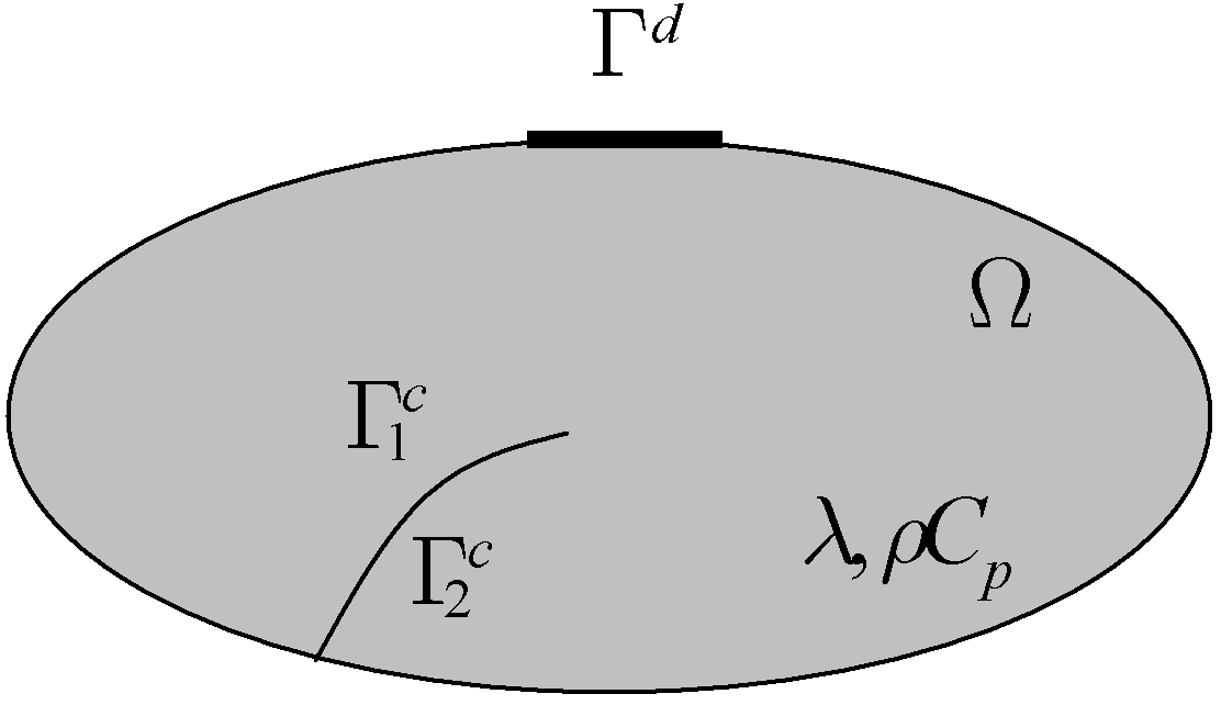
Figure 4.3-1: Notations
For the problem under consideration, noting \(\lambda\) and \(\rho {C}_{p}\) respectively the thermal conductivity coefficient and the volume heat at constant pressure, the heat equation is written as:
\(\mathrm{-}\mathrm{\nabla }\mathrm{.}(\lambda \mathrm{\nabla }T(x,t))\mathrm{=}\rho {C}_{p}\frac{\mathrm{\partial }T}{\mathrm{\partial }t}(x,t),\text{}\mathrm{\forall }(x,t)\mathrm{\in }\Omega \mathrm{\times }\left]{t}_{0},{t}_{f}\right]\) eq 4.3-1
notating:math: {T} _ {1}mathrm {=} {T} _ {text {|} {Gamma} _ {1} ^ {c}}, :math: {T} _ {1} _ {2}mathrm {=} {2} _ {T}} _ {text {| |} {Gamma} _ {2} ^ {c}}}, :math: {T} _ {2} _ {2} _ {T}}}, and:math: `h” `the heat exchange coefficient between the lips of the crack, the boundary conditions are written as:
\(\mathrm{\{}\begin{array}{c}T\mathrm{=}\stackrel{ˉ}{T}\text{sur}{\Gamma }^{d}\\ \lambda \frac{\mathrm{\partial }{T}_{1}}{\mathrm{\partial }{n}_{1}}\mathrm{=}h({T}_{2}\mathrm{-}{T}_{1})\text{sur}{\Gamma }_{1}^{c}\\ \lambda \frac{\mathrm{\partial }{T}_{2}}{\mathrm{\partial }{n}_{2}}\mathrm{=}h({T}_{1}\mathrm{-}{T}_{2})\text{sur}{\Gamma }_{2}^{c}\end{array}\) eq 4.3-2
with the the initial condition:
\(T(x,0)\mathrm{=}{T}_{0}(x),\text{}\mathrm{\forall }x\mathrm{\in }\Omega\)
The following functional areas are then introduced:
- math:
Vmathrm {=}left{vmathrm {in} {H} ^ {1} (Omega), {v} _ {text {|} {Gamma} ^ {d}}mathrm {d}}}mathrm {=}}mathrm {=}}mathrm {=}}stackrel {} {T}right}} `and:math: {V} _ {0}mathrm {0}} {0}mathrm =}left{vmathrm {in} {H} {H} ^ {1} (Omega), {v} _ {text {|} {Gamma} ^ {d}}}mathrm {in} {d}}}mathrm {=} 0right} `
The variational formulation associated with eq and eq is then written: find \(T\in V\) such as
\(\begin{array}{c}\phantom{\text{}\text{}\text{}\text{}\text{}}\underset{\Omega }{\mathrm{\int }}\rho {C}_{p}\frac{\mathrm{\partial }T}{\mathrm{\partial }t}vd\Omega +\underset{\Omega }{\mathrm{\int }}\lambda \mathrm{\nabla }T\mathrm{.}\mathrm{\nabla }vd\Omega \text{}\\ \text{}+\underset{{\Gamma }_{1}^{c}}{\mathrm{\int }}h({T}_{1}\mathrm{-}{T}_{2})vd\Gamma +\underset{{\Gamma }_{2}^{c}}{\mathrm{\int }}h({T}_{2}\mathrm{-}{T}_{1})vd\Gamma \mathrm{=}\mathrm{0,}\text{}\mathrm{\forall }v\mathrm{\in }{V}_{0}\end{array}\) eq 4.3-3
The time discretization is carried out by a \(\theta\) -diagram (see [bib 74]). We place ourselves between two successive time stakes \({t}_{n}\) and \({t}_{n+1}\), we note \(\Delta t\mathrm{=}{t}_{n+1}\mathrm{-}{t}_{n}\) the time step, and \(\theta \mathrm{\in }\mathrm{[}\mathrm{0,1}\mathrm{]}\) the parameter of the \(\theta\) -diagram. The following notations are then introduced:
\({T}^{\text{+}}\mathrm{=}T(x,{t}_{n+1})\), and \({T}^{\text{-}}\mathrm{=}T(x,{t}_{n})\)
- math:
{V} ^ {text {+}}mathrm {+}}mathrm {=}left{vmathrm {in} {H} ^ {1} (Omega), {v} _ {text {| | | | | | | | | | | | | text {| | | | | | | | | | | | | | | | |} | text {| | | | | | | | | | | | | | | | | | | | | | | | | |} | text {| | | | | | | | | | | | | | | | | | | | | | | | | | |} | | | | | | | | | | | | | | | | | | | | | | | | | | | | | | | | | |} and:math: {V} ^ {text {-}}mathrm {-}}mathrm {=}left{vmathrm {in} {H} ^ {1} (Omega), {v} _ {text {| | |}} {text {|}} {text {|}} {text {-}}mathrm {=}mathrm {=}stackrel {} {{T}} ^ {{T} ^ {text {| |}} {text {| |}} {text {|}} {text {|}} {text {|}} {text {-}}}}right}
Applying the \(\theta\) -schema to eq leads to the following variational formulation: given \({T}^{\text{-}}\in {V}^{\text{-}}\) find \({T}^{\text{+}}\in {V}^{\text{+}}\) such that
\(\begin{array}{c}\phantom{\text{}\text{}\text{}\text{}\text{}}\underset{\Omega }{\int }\rho {C}_{p}\frac{{T}^{\text{+}}}{\Delta t}vd\Omega +\underset{\Omega }{\int }\left(\theta \lambda \nabla {T}^{\text{+}}\mathrm{.}\nabla vd\Omega \right)\\ \text{}+\underset{{\Gamma }_{1}^{c}}{\int }\theta {h}^{\text{+}}({T}_{1}^{\text{+}}-{T}_{2}^{\text{+}})vd\Gamma +\underset{{\Gamma }_{2}^{c}}{\int }\theta {h}^{\text{+}}({T}_{2}^{\text{+}}-{T}_{1}^{\text{+}})vd\Gamma \\ \text{}=\underset{\Omega }{\int }\rho {C}_{p}\frac{{T}^{\text{-}}}{\Delta t}vd\Omega -\underset{\Omega }{\int }\left((1-\theta )\lambda \nabla {T}^{\text{-}}\mathrm{.}\nabla vd\Omega \right)\\ \text{}\phantom{\text{}}+\underset{{\Gamma }_{1}^{c}}{\int }(1-\theta ){h}^{\text{-}}({T}_{2}^{\text{-}}-{T}_{1}^{\text{-}})vd\Gamma +\underset{{\Gamma }_{2}^{c}}{\int }(1-\theta ){h}^{\text{-}}({T}_{1}^{\text{-}}-{T}_{2}^{\text{-}})vd\Gamma ,\text{}\forall v\in {V}_{0}\end{array}\) eq 4.3-4
4.4. X- FEM approximation of the temperature field#
We use the notations previously adopted for mechanics in paragraph 3.2 « Enrichissement de l’approximation du déplacement ». We recall the classical finite element approximation:
\({T}^{h}(x)=\sum _{i\in {N}_{n}(x)}{T}_{i}{\mathrm{\phi }}_{i}(x)\)
For its part, the enriched approximation is written as:
\({T}^{h}(x)=\sum _{i\in {N}_{n}(x)}{T}_{i}^{C}{\mathrm{\phi }}_{i}(x)+\sum _{j\in {N}_{n}(x)\cap K}{T}_{j}^{H}{\mathrm{\phi }}_{j}(x){H}_{j}\left(\mathit{lsn}(x)\right)+\sum _{k\in {N}_{n}(x)\cap L}{T}_{k}^{\mathit{CT}}{\mathrm{\phi }}_{k}(x){F}^{1}\left(\mathit{lsn}(x),\mathit{lst}(x)\right)\)
This expression is composed of 3 terms. The 1st term is the classical term where \({T}_{i}^{C}\) denotes the classical degrees of freedom, the second term is the term enriched by the \({H}_{j}\) domain selection function with \({T}_{j}^{H}\) the corresponding enriched degrees of freedom, and the third term is the term enriched by the singular function \({F}^{1}\) (« Crack-Tip » enrichment) with \({T}_{k}^{\mathit{CT}}\) the corresponding enriched degrees of freedom.
It is assumed that the domain is partitioned \(\mathrm{\Omega }\) by the crack interface of the crack \({\Gamma }^{c}\) into two domains \({\mathrm{\Omega }}_{\text{-}}\) on the side of \({\Gamma }_{1}^{c}\) and \({\mathrm{\Omega }}_{\text{+}}\) on the side of \({\mathrm{\Gamma }}_{2}^{c}\).
Below is the expression for \({H}_{j}\):
\(\mathit{Si}\phantom{\rule{2em}{0ex}}{x}_{j}\in {\mathrm{\Omega }}_{\text{+}},\phantom{\rule{2em}{0ex}}{H}_{j}(x)=\{\begin{array}{c}\phantom{\rule{2em}{0ex}}0\phantom{\rule{2em}{0ex}}\text{si}\phantom{\rule{0.5em}{0ex}}x\in {\mathrm{\Omega }}_{\text{+}}\\ -2\phantom{\rule{2em}{0ex}}\text{si}\phantom{\rule{0.5em}{0ex}}x\notin {\mathrm{\Omega }}_{\text{+}}\end{array}\) \(\mathit{Si}\phantom{\rule{2em}{0ex}}{x}_{j}\in {\mathrm{\Omega }}_{\text{-}},\phantom{\rule{2em}{0ex}}{H}_{j}(x)=\{\begin{array}{c}\phantom{\rule{2em}{0ex}}0\phantom{\rule{2em}{0ex}}\text{si}\phantom{\rule{0.5em}{0ex}}x\in {\mathrm{\Omega }}_{\text{-}}\\ +2\phantom{\rule{2em}{0ex}}\text{si}\phantom{\rule{0.5em}{0ex}}x\notin {\mathrm{\Omega }}_{\text{-}}\end{array}\)
Below is the expression for \({F}^{1}\):
\({F}^{1}(\mathit{lsn}(x),\mathit{lst}(x))=\sqrt{r}\text{sin}\frac{\theta }{2}\)
where \((r,\theta )\) are the polar coordinates in the local base at the crack bottom determined from level-sets \((\mathit{lsn}(x),\mathit{lst}(x))\).
Note:
In mechanics, four functions determined from the asymptotic development of the displacement field at the bottom of a crack are introduced into the term of singular enrichment. In thermal, only the function \({F}^{1}\) is introduced, which is the only function (among the four) that is discontinuous across the crack. This type of enrichment, retained in [bib 75 ] in the case of a zero flow condition imposed on the lips of the crack (adiabatic crack), is here introduced for the case of an adiabatic crack as for the case of an exchange condition between the lips of the crack.
4.5. Integration of matrices and elementary vectors#
This paragraph details the expression of the elementary quantities associated with each term of the variational formulation eq of the time-discretized linear thermal problem.
4.5.1. Volume integrals#
Let \(E\) be an X- FEM thermal element. We denote \({\{\text{T}\}}_{E}^{T}\), \({[\text{N}]}_{E}\) and \({[\text{B}]}_{E}\) respectively the elementary vector of the nodal unknowns (at time \(\text{+}\)), the elementary matrix of shape functions and the elementary matrix of the derivatives of the derivatives of the shape functions. As an example, we can consider an element of dimension \({n}_{\mathit{dim}}=2\text{ou}3\), with \(n\) nodes, and of the « Heaviside/Crack-Tip » type. \({\{\text{T}\}}_{E}^{T}\), \({[\text{N}]}_{E}\), and \({[\text{B}]}_{E}\) are written in this case:
\({\{\text{T}\}}_{E}^{T}=\left[{T}_{1}^{C}\text{}{T}_{1}^{H}\text{}{T}_{1}^{\mathit{CT}}\text{...}{T}_{n}^{C}\text{}{T}_{n}^{H}\text{}{T}_{n}^{\mathit{CT}}\right]\) in size \(\mathrm{3n}\)
\({[\text{N}]}_{E}=\left[{N}_{1}\text{}{H}_{1}{N}_{1}\text{}{F}^{1}{N}_{1}\text{...}{N}_{n}\text{}{H}_{n}{N}_{n}\text{}{F}^{1}{N}_{n}\right]\) in size \((\mathrm{1,3}n)\)
\({[\text{B}]}_{E}=\left[\nabla {N}_{1}\text{}\nabla ({H}_{1}{N}_{1})\text{}\nabla ({F}^{1}{N}_{1})\text{...}\nabla {N}_{n}\text{}\nabla ({H}_{n}{N}_{n})\text{}\nabla ({F}^{1}{N}_{n})\right]\) in size \(({n}_{\mathit{dim}}\mathrm{,3}n)\)
All the volume quantities are integrated according to the procedure based on the division into sub-elements, and detailed in the case of mechanics on page 89. The expression for these elementary quantities is given below.
mass matrix (option MASS_THER ) :
\(\underset{E}{\int }\frac{\rho {C}_{p}}{\Delta t}{[\text{N}]}_{E}^{T}{[\text{N}]}_{E}d\Omega\)
stiffness matrix (option RIGI_THER ) :
\(\underset{E}{\int }\theta \lambda {[\text{B}]}_{E}^{T}{[\text{B}]}_{E}d\Omega\)
vector relating to time discretization (option CHAR_THER_EVOL ) :
\(\underset{E}{\int }\frac{\rho {C}_{p}}{\Delta t}{[\text{N}]}_{E}^{T}{[\text{N}]}_{E}{\{{\text{T}}^{\text{-}}\}}_{E}d\Omega -\underset{E}{\int }(1-\theta )\lambda {[\text{B}]}_{E}^{T}{[\text{B}]}_{E}{\{{\text{T}}^{\text{-}}\}}_{E}d\Omega\)
4.5.2. Surface integrals#
These quantities correspond to the condition of heat exchange between the lips of the crack, and are integrated along the lips of the crack according to the procedure based on the discretization of the lips into « contact facets ». This procedure is detailed in the case of mechanics on page 93.
First of all, the elementary matrices \({[\stackrel{̃}{{\text{N}}_{1}}]}_{E}\) and \({[\stackrel{̃}{{\text{N}}_{2}}]}_{E}\), defined as the matrices of the traces of the shape functions on \({\Gamma }_{1}^{c}\) and \({\Gamma }_{2}^{c}\) respectively, are introduced:
- math:
{[stackrel {}} {{text {N}} {{text {N}}}} _ {E} = {[{text {N}} _ {text {| |} {Gamma} _ {Gamma} _ {1}} _ {c}} _ {c}}]} _ {c}}]} _ {c}}]} _ {c}}]} _ {c}}]} _ {C}}]} _ {C}}]} _ {E}text {,} {{text {N}} | {{text {N}} | {| Gamma} _ {2}}]} _ {E} = {[{text {N}}} _ {text {N}}} _ {Gamma} _ {2} ^ {c}}]]}} _ {E}
Note:
From one matrix to another, the coefficients corresponding to classical enrichment are equal, and the coefficients corresponding to Heaviside and « Crack-Tip » enrichment are linked by::math: {H} _ {text {|} {text {| |} {mathrm {Gamma}} {mathrm {Gamma}}} {mathrm {Gamma}}} _ {1} _ {1} ^ {c}} =2, and:math:` {F} _ {text {|} {mathrm {Gamma}} _ {2} ^ {c}} ^ {1} - {F} _ {F} _ {text {|} _ {text {| |}} {\ text {|}} {text {|}} _ {1} ^ {c}} ^ {1} =2 {F}} _ {F} _ {text {| |}mathrm {Gamma}} _ {1} ^ {c}} ^ {1} *because the polar angle is*:math: `mathrm {pm}pi.
The following coupling matrices are then introduced:
\({\mathrm{[}\tilde{{\text{N}}_{12}}\mathrm{]}}_{E}\mathrm{=}{\mathrm{[}\tilde{{\text{N}}_{1}}\mathrm{]}}_{E}\mathrm{-}{\mathrm{[}\tilde{{\text{N}}_{2}}\mathrm{]}}_{E}\text{,}{\mathrm{[}\tilde{{\text{N}}_{21}}\mathrm{]}}_{E}\mathrm{=}{\mathrm{[}\tilde{{\text{N}}_{2}}\mathrm{]}}_{E}\mathrm{-}{\mathrm{[}\tilde{{\text{N}}_{1}}\mathrm{]}}_{E}\)
The elementary quantities are then given by the following expressions, with \({\Gamma }_{E}^{c}\) the set of facets constituting the discretization of the crack within the element \(E\):
matrix relating to the exchange condition (option RIGI_THER_PARO_R ) :
\(\underset{{\Gamma }_{E}^{c}}{\mathrm{\int }}\theta {h}^{\text{+}}{\mathrm{[}\tilde{{\text{N}}_{1}}\mathrm{]}}_{E}^{T}{\mathrm{[}\tilde{{\text{N}}_{12}}\mathrm{]}}_{E}d\Gamma +\underset{{\Gamma }_{E}^{c}}{\mathrm{\int }}\theta {h}^{\text{+}}{\mathrm{[}\tilde{{\text{N}}_{2}}\mathrm{]}}_{E}^{T}{\mathrm{[}\tilde{{\text{N}}_{21}}\mathrm{]}}_{E}d\Gamma\)
vector relating to the exchange condition (option CHAR_THER_PARO_R ) :
\(\underset{{\Gamma }_{E}^{c}}{\mathrm{\int }}(1\mathrm{-}\theta ){h}^{\text{-}}{\mathrm{[}\tilde{{\text{N}}_{1}}\mathrm{]}}_{E}^{T}{\mathrm{[}\tilde{{\text{N}}_{21}}\mathrm{]}}_{E}{\mathrm{\{}{\text{T}}^{\text{-}}\mathrm{\}}}_{E}d\Gamma +\underset{{\Gamma }_{E}^{c}}{\mathrm{\int }}(1\mathrm{-}\theta ){h}^{\text{-}}{\mathrm{[}\tilde{{\text{N}}_{2}}\mathrm{]}}_{E}^{T}{\mathrm{[}\tilde{{\text{N}}_{12}}\mathrm{]}}_{E}{\mathrm{\{}{\text{T}}^{\text{-}}\mathrm{\}}}_{E}d\Gamma\)