5. Energy calculation of Stress Intensity Factors

This part recalls the \(G\) -theta method used in Code_Aster for calculating the energy return rate in linear fracture mechanics, following a classical finite element calculation (in 2D or 3D). This method is also used to calculate stress intensity factors, using the bilinear form of \(g\) but only in 2D. Because to be able to use it in 3D, you need to know the local base at the bottom of the crack in order to express the asymptotic fields as a function of polar coordinates \((r,\theta )\).

Next, we present the contribution of classical finite element level sets, which was to be able to build a local base at the bottom of a crack in 3D. As we saw in paragraph [§ 2.3], the gradients of the level sets give a local base to the crack bottom. Moreover, the polar coordinates in this local base are easily expressed according to the level sets (see Figure 3.2.3-1). Thus, thanks to the level sets, the \(G\) -theta method was applicable to the calculation of stress intensity factors in 3D with classical finite elements. In this context, the crack is meshed, a classical calculation is carried out. In post-processing, the two level-set fields are determined from the meshed crack and a discretization of the crack background is deduced. The theta field is constructed from this discretized crack background, and the \(G\) -theta method is applied.

The last point is the calculation of the energy return rate and the stress intensity factors, following an X- FEM calculation. In this case, the crack is not meshed, but the procedure followed is almost the same: the discretization of the crack background is determined from the level sets, a theta field is constructed and the \(G\) -theta is applied. The only difference is in terms of digital integrations: with X- FEM, digital integrations require a sub-division of the elements to be integrated. In fact, the sub-division carried out is used to calculate tangent matrices and second members.

5.1. G-theta method for calculating G

5.1.1. Equilibrium relationships

In linear elasticity, we define the free energy density \(\Psi\), in the absence of deformations and initial stresses, by a definite positive quadratic form of the components of the deformation tensor:

\(\Psi (\varepsilon ,T)\mathrm{=}\frac{1}{2}(\varepsilon \mathrm{-}{\varepsilon }^{\text{th}})\mathrm{:}C\mathrm{:}(\varepsilon \mathrm{-}{\varepsilon }^{\text{th}})\)

\(C\) is the Hooke tensor (4th order tensor), and the two dots denote the tensor product contracted on two indices.

The stress tensor \(\sigma\) derives from the potential \(\Psi\) to give the state law (or material behavior law):

\(\sigma \mathrm{=}\frac{\mathrm{\partial }\Psi }{\mathrm{\partial }\varepsilon }(\varepsilon ,T)\mathrm{=}C\mathrm{:}(\varepsilon \mathrm{-}{\varepsilon }^{\text{th}})\)

Equilibrium relationships in weak formulations are obtained by minimizing the overall potential energy of the system:

\(W(v)\mathrm{=}\underset{\Omega }{\mathrm{\int }}\Psi (\varepsilon (v))d\Omega \mathrm{-}\underset{\Omega }{\mathrm{\int }}{f}_{i}{v}_{i}d\Omega \mathrm{-}\underset{S}{\mathrm{\int }}{g}_{i}{v}_{i}d\Gamma\)

This function being minimal for the displacement field \(u\):

\(\begin{array}{c}\delta W\mathrm{=}\underset{\Omega }{\mathrm{\int }}\frac{\mathrm{\partial }\Psi }{\mathrm{\partial }{\varepsilon }_{\text{ij}}}\delta {\varepsilon }_{\text{ij}}d\Omega \mathrm{-}\underset{\Omega }{\mathrm{\int }}{f}_{i}\delta {v}_{i}d\Omega \mathrm{-}\underset{S}{\mathrm{\int }}{g}_{i}\delta {v}_{i}d\Gamma \\ \mathrm{=}\underset{\Omega }{\mathrm{\int }}{\sigma }_{\text{ij}}\frac{1}{2}(\delta {v}_{i,j}+\delta {v}_{j,i})d\Omega \mathrm{-}\underset{\Omega }{\mathrm{\int }}{f}_{i}\delta {v}_{i}d\Omega \mathrm{-}\underset{S}{\mathrm{\int }}{g}_{i}\delta {v}_{i}d\Gamma \\ \mathrm{=}\underset{\Omega }{\mathrm{\int }}{\sigma }_{\text{ij}}\delta {v}_{i,j}d\Omega \mathrm{-}\underset{\Omega }{\mathrm{\int }}{f}_{i}\delta {v}_{i}d\Omega \mathrm{-}\underset{S}{\mathrm{\int }}{g}_{i}\delta {v}_{i}d\Gamma \mathrm{=}0\end{array}\)

Equilibrium relationships in weak formulations are therefore written as follows:

Find \(u\in V\) such as

\(\underset{\Omega }{\mathrm{\int }}{\sigma }_{\text{ij}}{v}_{\text{i,j}}d\Omega \mathrm{=}\underset{\Omega }{\mathrm{\int }}{f}_{i}{v}_{i}d\Omega +\underset{S}{\mathrm{\int }}{g}_{i}{v}_{i}d\Gamma ,\mathrm{\forall }v\mathrm{\in }{V}_{0}\)

5.1.2. Lagrangian expression for the rate of energy restoration

By definition, the local energy recovery rate \(G\) is defined by the opposite of the derivative of potential energy with respect to the domain:

\(G\mathrm{=}\mathrm{-}\frac{\mathrm{\partial }W}{\mathrm{\partial }\Omega }\)

The virtual extensions method used here is a Lagrangian method for deriving potential energy. It consists in introducing transformations:

\({F}^{\eta }\mathrm{:}P\mathrm{\in }\Omega \to M\mathrm{=}P+\eta \theta (P)\mathrm{\in }{\Omega }^{\eta }\)

which, to each material point \(P\) of the reference domain \(O\), associate a spatial point \(M\) of the transformed domain \({\Omega }^{\eta }\). These transformations, representing the propagation of the crack, should only modify the position of the bottom of crack \({\Gamma }_{0}\). Fields \(\theta\) must be tangent to the surface of the crack.

Let \(n\) be normal to the surface of the crack, fields \(\theta\) must check:

\({\theta }_{j}{n}_{j}\mathrm{=}0\text{sur}{\Gamma }_{\text{cr}}\)

Let \(m\) be the unit normal at the crack bottom, located in the tangential plane of the crack.

According to [bib 50], the local energy restoration rate \(G\) is a solution of the following variational equation:

\(\underset{{\Gamma }_{0}}{\mathrm{\int }}G\theta \mathrm{\cdot }m\mathrm{=}G(\theta ),\mathrm{\forall }\theta \mathrm{\in }\theta\) eq. 5.1.2-1

where \(G(\theta )\) is defined by the opposite of the derivative of the potential energy \(W(u(\eta ))\) at equilibrium with respect to the initial evolution of the crack bottom:

\(G(\theta )\mathrm{=}\mathrm{-}{\frac{\text{dW}(u(\eta ))}{d\eta }\mathrm{\mid }}_{\eta \mathrm{=}0}\) (particulate derivative)

To derive the potential energy with respect to its support (in the vicinity of the reference support), we use the Reynolds transport theorem:

For a \({F}^{\eta }\) transformation of class \({C}^{1}\) and a function \(\varphi\) (tensor of order 0, 1 or 2) of class \({C}^{1}\), by noting \(\dot{\varphi }\) the Lagrangian derivative linked to the domain variation, we have the following relationship:

\({\frac{\mathrm{\partial }}{\mathrm{\partial }\eta }(\underset{\Omega }{\mathrm{\int }}\varphi d\Omega )\mathrm{\mid }}_{\eta \mathrm{=}0}\mathrm{=}\underset{\Omega }{\mathrm{\int }}\dot{\varphi }+\varphi \text{div}{(\frac{\mathrm{\partial }{F}^{\eta }}{\mathrm{\partial }\eta })}_{\eta \mathrm{=}0}d\Omega\)

In fact, in practice, the \({F}^{\eta }\) transform is not always of class \({C}^{1}\) because the field \(\theta\) is only \({C}^{1}\) piecewise.

So

\(\begin{array}{ccc}\mathrm{-}G(\theta )& \text{=}& {\frac{\mathrm{\partial }}{\mathrm{\partial }\eta }(\underset{\Omega }{\mathrm{\int }}\Psi \mathrm{-}{f}_{i}{u}_{i}d\Omega \mathrm{-}\underset{S}{\mathrm{\int }}{g}_{i}{u}_{i}d\Gamma )\mathrm{\mid }}_{\eta \mathrm{=}0}\\ & \text{=}& \underset{\Omega }{\mathrm{\int }}\stackrel{\mathrm{\cdot }}{\stackrel{}{\Psi \mathrm{-}{f}_{i}{u}_{i}}}+(\Psi \mathrm{-}{f}_{i}{u}_{i})\text{div}(\theta )d\Omega \mathrm{-}{\mathrm{\int }}_{S}\stackrel{\mathrm{\cdot }}{\stackrel{}{{g}_{i}{u}_{i}}}+{g}_{i}{u}_{i}(\text{div}(\theta )\mathrm{-}\frac{\mathrm{\partial }\theta }{\mathrm{\partial }{n}_{k}}{n}_{k})d\Gamma \end{array}\)

where:

\(\Psi (\varepsilon ,T)=\frac{1}{2}\lambda {({\epsilon }_{\mathrm{ii}})}^{2}+\mu {\varepsilon }_{\mathrm{ij}}{\varepsilon }_{\mathrm{ij}}-3K\alpha (T-{T}_{\mathrm{réf}})\)

\(\dot{\Psi }(\epsilon )=\frac{\partial \Psi }{\partial {\epsilon }_{\text{ij}}}{\dot{\epsilon }}_{\text{ij}}+\frac{\partial \Psi }{\partial T}\dot{T}={\sigma }_{\text{ij}}{\dot{\epsilon }}_{\text{ij}}+\frac{\partial \Psi }{\partial T}\dot{T}\)

So:

\(\begin{array}{c}\mathrm{-}G(\theta )\mathrm{=}\underset{\Omega }{\mathrm{\int }}{\sigma }_{\text{ij}}{\dot{\varepsilon }}_{\text{ij}}+\frac{\mathrm{\partial }\Psi }{\mathrm{\partial }T}\dot{T}\mathrm{-}{\dot{f}}_{i}{u}_{i}\mathrm{-}{f}_{i}{\dot{u}}_{i}+(\Psi \mathrm{-}{f}_{i}{u}_{i}){\theta }_{k,k}d\Omega \\ \mathrm{-}\underset{S}{\mathrm{\int }}{\dot{g}}_{i}{u}_{i}\mathrm{-}{g}_{i}{\dot{u}}_{i}+{g}_{i}{u}_{i}({\theta }_{k,k}\mathrm{-}\frac{\mathrm{\partial }\theta }{\mathrm{\partial }{n}_{k}}{n}_{k})d\Gamma \end{array}\)

First, let’s use the relationship giving the Lagrangian derivative of a \(\varphi\) field as a function of its Eulerian derivative \(\frac{\mathrm{\partial }\varphi }{\mathrm{\partial }\eta }\):

\(\dot{\varphi }\mathrm{=}\frac{\mathrm{\partial }\varphi }{\mathrm{\partial }\eta }+\mathrm{\nabla }\varphi \mathrm{\cdot }\theta\)

According to this relationship, the volume force \(f\) being assumed to be independent of \(\eta\), i.e. being the restriction to \(O\) of fields defined on \({ℝ}^{3}\), we can write that \(\frac{\partial {f}_{i}}{\partial \eta }=0\). As is the same for \(g\) and \(T\), we have the following relationships:

\(\begin{array}{c}\dot{T}\mathrm{=}{T}_{,k}{\theta }_{k}\\ {\dot{f}}_{i}\mathrm{=}{f}_{i,k}{\theta }_{k}\\ {\dot{g}}_{i}\mathrm{=}{g}_{i,k}{\theta }_{k}\end{array}\)

Second, let’s use the relationship giving the Lagrangian derivative of the field gradient as a function of the field gradient and the field derivative gradient:

\(\dot{\mathrm{\nabla }}\varphi \mathrm{=}\mathrm{\nabla }\dot{\varphi }\mathrm{-}\mathrm{\nabla }\varphi \mathrm{\cdot }\mathrm{\nabla }\theta\)

or in index notations,

\(\stackrel{\mathrm{\cdot }}{\stackrel{}{{\varphi }_{i,j}}}\mathrm{=}{\dot{\varphi }}_{i,j}\mathrm{-}{\varphi }_{i,p}{\theta }_{p,j}\)

therefore

\({\dot{\varepsilon }}_{i,j}\mathrm{=}\frac{1}{2}({\dot{u}}_{i,j}+{\dot{u}}_{j,i})\mathrm{-}\frac{1}{2}({u}_{i,p}{\theta }_{p,j}+{u}_{j,p}{\theta }_{p,i})\)

We replace the 2 expressions in the first and we get:

\(\begin{array}{c}\mathrm{-}G(\theta )\mathrm{=}\underset{\Omega }{\mathrm{\int }}{\sigma }_{\text{ij}}{\dot{u}}_{i,j}+\frac{\mathrm{\partial }\Psi }{\mathrm{\partial }T}{T}_{,k}{\theta }_{k}\mathrm{-}{\sigma }_{\text{ij}}{u}_{i,p}{\theta }_{p,j}\mathrm{-}{f}_{i,k}{\theta }_{k}{u}_{i}\mathrm{-}{f}_{i}{\dot{u}}_{i}+(\Psi \mathrm{-}{f}_{i}{u}_{i}){\theta }_{k,k}d\Omega \\ \mathrm{-}\underset{S}{\mathrm{\int }}{g}_{i,k}{\sigma }_{k}{u}_{i}\mathrm{-}{g}_{i}{\dot{u}}_{i}+{g}_{i}{u}_{i}({\theta }_{k,k}\mathrm{-}\frac{\mathrm{\partial }\sigma }{\mathrm{\partial }{n}_{k}}{n}_{k})d\Gamma \end{array}\)

We can eliminate the terms in \(\dot{u}\) by noting that field \(\dot{u}\) is kinematically admissible and satisfies the equilibrium equation:

\(\underset{\Omega }{\mathrm{\int }}{\sigma }_{\text{ij}}{\dot{u}}_{i,j}d\Omega \mathrm{=}\underset{\Omega }{\mathrm{\int }}{f}_{i}{\dot{u}}_{i}d\Omega +\underset{S}{\mathrm{\int }}{g}_{i}{\dot{u}}_{i}d\Gamma\)

This results in the final expression for \(J(\theta )\):

\(\begin{array}{c}G(\theta )\mathrm{=}\underset{\Omega }{\mathrm{\int }}{\sigma }_{\text{ij}}{u}_{i,p}{\theta }_{p,j}\mathrm{-}\Psi {\theta }_{k,k}+\frac{\mathrm{\partial }\Psi }{\mathrm{\partial }T}{T}_{,k}{\theta }_{k}d\Omega \\ +\underset{\Omega }{\mathrm{\int }}{f}_{i,k}{\theta }_{k}{u}_{i}+{f}_{i}{u}_{i}{\theta }_{k,k}d\Omega \\ +\underset{S}{\mathrm{\int }}{g}_{i,k}{\theta }_{k}{u}_{i}+{g}_{i}{u}_{i}({\theta }_{k,k}\mathrm{-}\frac{\mathrm{\partial }\theta }{\mathrm{\partial }{n}_{k}}{n}_{k})d\Gamma \end{array}\) eq. 5.1.2-2

Note:

This form of the integral \(J\) does not use contour integrals but domain integrals.

5.1.3. Discretizations

Note \(s\) the curvilinear abscissa at the bottom of the crack. Calculating the local value of \(G\) requires solving the following variational equation for several \({\theta }^{i}\) fields:

\({\mathrm{\int }}_{{\Gamma }_{0}}G(s){\theta }^{i}(s)\mathrm{\cdot }m(s)\text{ds}\mathrm{=}G({\theta }^{i})\mathrm{\forall }i\mathrm{\in }\mathrm{[}\mathrm{1,}P\mathrm{]}\)

The scalar field \(G(s)\) is discretized on a basis noted \({({p}_{j}(s))}_{1\le j\le N}\):

\(G(s)\mathrm{=}\mathrm{\sum }_{j\mathrm{=}1}^{N}{G}_{j}{p}_{j}(s)\)

Likewise, fields \({\theta }^{i}\) are discretized on a basis marked \({({q}_{k}(s))}_{1\le k\le M}\). Let \({\stackrel{ˉ}{\theta }}^{i}\) be the trace of the \({\theta }^{i}\) field on the bottom of the crack \({\Gamma }_{0}\): \({\stackrel{ˉ}{\theta }}^{i}(s)\mathrm{=}{\theta \mathrm{\mid }}_{{\Gamma }_{0}}(s)\) and where \({\theta }_{k}^{i}\) be the components of \({\stackrel{ˉ}{\theta }}^{i}(s)\) in this base:

\({\stackrel{ˉ}{\theta }}^{i}(s)\mathrm{=}\mathrm{\sum }_{k\mathrm{=}1}^{M}{\theta }_{k}^{i}{q}_{k}(s)\) eq. 5.1.3-1

By injecting these expressions into the variational equation, it comes:

\(\underset{{\Gamma }_{0}}{\mathrm{\int }}\mathrm{\sum }_{j\mathrm{=}1}^{N}{G}_{j}{p}_{j}(s)\mathrm{\sum }_{k\mathrm{=}1}^{M}({\theta }_{k}^{i}{q}_{k}(s))\mathrm{\cdot }m(s)\mathit{ds}\mathrm{=}G({\theta }^{i}),\mathrm{\forall }i\mathrm{\in }\mathrm{[}\mathrm{1,}P\mathrm{]}\)

The \({G}_{j}\) can therefore be determined by solving the linear system with \(P\) equations and \(N\) unknowns:

\(\mathrm{\{}\begin{array}{c}\mathrm{\sum }_{j\mathrm{=}1}^{N}{a}_{\mathit{ij}}{G}_{j}\mathrm{=}{b}_{i},i\mathrm{=}\mathrm{1,}P\\ \text{avec}{a}_{\mathit{ij}}\mathrm{=}\mathrm{\sum }_{k\mathrm{=}1}^{M}{\theta }_{k}^{i}\underset{{\Gamma }_{0}}{\mathrm{\int }}{p}_{j}(s){q}_{k}(s)\mathrm{\cdot }m(s)\mathit{ds}\\ \phantom{\mathit{avec}}{b}_{i}\mathrm{=}G({\theta }^{i})\end{array}\)

This system has a solution if we choose \(P\) \({\theta }^{i}\) independent fields such as: \(P\ge N\) and if \(M\ge N\). It may have more equations than unknowns, in which case it is solved in a least-squares sense.

5.2. G-theta method for calculating KI, KII and KIII with level sets

This paragraph presents the contribution of level sets for the calculation of stress intensity factors in 3D. It is based on the separation of mixed modes using the bilinear form of \(g\). This bilinear form is used in*Code_Aster* for the calculation by the \(G\) -theta method of \({K}_{I}\), \({K}_{\mathit{II}}\) in 2D [bib 49].

5.2.1. Bilinear form of g

The calculation of stress intensity factors can also be done using the theta method, by defining a symmetric bilinear form \(g\) with:

\(g(u,v)\mathrm{=}\frac{1}{4}(G(u+v)\mathrm{-}G(u\mathrm{-}v))\) eq. 5.2.1-1

Thus, being two displacement fields \(u\) and \(v\), the calculation of \(g(u,v)\) is performed using the expression for \(G\) given by the equation [eq.], in which the deformations related to \(u\) and \(v\) derive from the fields \(u\) and \(v\), and the constraints linked to \(u\) and \(v\) are deduced by the law of behavior:

\(\begin{array}{c}\varepsilon (u)\mathrm{=}{\mathrm{\nabla }}_{s}u,\varepsilon (v)\mathrm{=}{\mathrm{\nabla }}_{s}v\\ \sigma (u)\mathrm{=}C\mathrm{:}\varepsilon (u),\sigma (v)\mathrm{=}C\mathrm{:}\varepsilon (v)\end{array}\)

Using the notations from [bib 49], the classic \(J(\theta )\) term [eq.] is:

\(\begin{array}{c}\text{TCLA}\mathrm{=}\sigma (u)\mathrm{:}(\mathrm{\nabla }u\mathrm{\nabla }\theta )\mathrm{-}\Psi (\varepsilon (u))\text{div}\theta \\ \mathrm{=}(\mathit{S2}\mathrm{-}\mathit{S2}\text{TH})\mathrm{-}\frac{1}{2}(\mathit{S1}\mathrm{-}\mathit{S1}\text{TH})\text{div}\theta \end{array}\)

We recall that in elasticity, free energy is expressed as a function of Lamé coefficients \(\lambda\) and \(\mu\):

\(\begin{array}{c}\Psi \mathrm{=}\frac{1}{2}\lambda {({\varepsilon }_{\text{ii}})}^{2}+\mu {\varepsilon }_{\text{ij}}{\varepsilon }_{\text{ij}}\mathrm{-}{\Psi }^{\text{th}}\\ \phantom{\Psi }\mathrm{=}\frac{1}{2}\left[(\lambda +2\mu )({\varepsilon }_{\text{11}}^{2}+{\varepsilon }_{\text{22}}^{2}+{\varepsilon }_{\text{33}}^{2})+2\lambda ({\varepsilon }_{\text{11}}{\varepsilon }_{\text{22}}+{\varepsilon }_{\text{11}}{\varepsilon }_{\text{33}}+{\varepsilon }_{\text{22}}{\varepsilon }_{\text{33}})+2\mu (2{\varepsilon }_{\text{12}}^{2}+2{\varepsilon }_{\text{13}}^{2}+2{\varepsilon }_{\text{23}}^{2})\right]\mathrm{-}{\Psi }^{\text{th}}\end{array}\)

with \({\Psi }^{\text{th}}\mathrm{=}\mathrm{3K}\alpha (T\mathrm{-}{T}^{\text{ref}})\text{tr}\varepsilon\)

For each term \(\mathrm{S1}\) and \(\mathrm{S2}\), we will first write their usual expression, then we will move on to the bilinear form.

5.2.1.1. Expression of S1 and S1TH

We write \(\mathrm{S1}\) with the following expression:

\(\mathit{S1}\mathrm{=}\mathit{C1}\text{.}S\text{11}+\mathit{C2}\text{.}S\text{12}+\mathit{C3}\text{.}S\text{13}\)

by asking:

\(\mathrm{\{}\begin{array}{c}\mathit{C1}\mathrm{=}\lambda +2\mu \\ \mathit{C2}\mathrm{=}\lambda \\ \mathit{C3}\mathrm{=}\mu \end{array}\) and \(\begin{array}{c}S\text{11}\mathrm{=}{u}_{\mathrm{1,1}}^{2}+{u}_{\mathrm{2,2}}^{2}+{u}_{\mathrm{3,3}}^{2}\\ S\text{12}\mathrm{=}2({u}_{\mathrm{1,1}}{u}_{\mathrm{2,2}}+{u}_{\mathrm{1,1}}{u}_{\mathrm{3,3}}+{u}_{\mathrm{2,2}}{u}_{\mathrm{3,3}})\\ S\text{13}\mathrm{=}{({u}_{\mathrm{1,2}}+{u}_{\mathrm{2,1}})}^{2}+{({u}_{\mathrm{1,3}}+{u}_{\mathrm{3,1}})}^{2}+{({u}_{\mathrm{2,3}}+{u}_{\mathrm{3,2}})}^{2}\end{array}\)

Now let’s write the associated bilinear form. Free energy then depends on two fields \(u\) and \(v\). The material coefficients \(\mathrm{C1}\), \(\mathrm{C2}\) and \(\mathrm{C3}\) are obviously unchanged, and the new coefficients \(S\text{11}\), \(S\text{12}\) and \(S\text{13}\) have the following expressions:

\(\begin{array}{}S\text{11}={u}_{\mathrm{1,1}}{v}_{\mathrm{1,1}}+{u}_{\mathrm{2,2}}{v}_{\mathrm{2,2}}+{u}_{\mathrm{3,3}}{v}_{\mathrm{3,3}}\\ S\text{12}=({u}_{\mathrm{1,1}}{v}_{\mathrm{2,2}}+{u}_{\mathrm{2,2}}{v}_{\mathrm{1,1}})+({u}_{\mathrm{1,1}}{v}_{\mathrm{3,3}}+{u}_{\mathrm{3,3}}{v}_{\mathrm{1,1}})+({u}_{\mathrm{2,2}}{u}_{\mathrm{3,3}}+{u}_{\mathrm{3,3}}{v}_{\mathrm{2,2}})\\ S\text{13}=({u}_{\mathrm{1,2}}+{u}_{\mathrm{2,1}})({v}_{\mathrm{1,2}}+{v}_{\mathrm{2,1}})+({u}_{\mathrm{1,3}}+{u}_{\mathrm{3,1}})({v}_{\mathrm{1,3}}+{v}_{\mathrm{3,1}})+({u}_{\mathrm{2,3}}+{u}_{\mathrm{3,2}})({v}_{\mathrm{2,3}}+{v}_{\mathrm{3,2}})\end{array}\)

The expression for the thermal part is:

\(\text{SITH}=3K\alpha (({T}_{u}-{T}_{\text{réf}})\text{tr}\epsilon (v)+({T}_{v}-{T}_{\text{réf}})\text{tr}\epsilon (u))\)

For the calculation of \({K}_{i}\), \(v\) is the asymptotic field in mode i, obtained for \({T}_{v}={T}_{\text{réf}}\), so the terms in \(({T}_{v}-{T}_{\text{réf}})\) are simplified:

\(\text{SITH}=3K\alpha (({T}_{u}-{T}_{\text{réf}})\text{tr}\epsilon (v))\)

5.2.1.2. Expression of S2 and S2TH

As with \(\mathrm{S1}\), we write \(\mathrm{S2}\) with the following expression:

\(\mathit{S2}\mathrm{=}\mathit{C1}\text{.}S\text{21}+\mathit{C2}\text{.}S\text{22}+\mathit{C3}\text{.}S\text{23}\)

The material coefficients \(\mathrm{C1}\), \(\mathrm{C2}\) and \(\mathrm{C3}\) are those defined in the preceding paragraph.

The expressions for the coefficients \(S\text{21}\), \(S\text{22}\) and \(S\text{23}\) are:

\(\begin{array}{c}\mathit{S21}\mathrm{=}\mathrm{\sum }_{k\mathrm{=}1}^{3}\mathrm{\sum }_{p\mathrm{=}1}^{3}{u}_{k,k}{u}_{k,p}{\theta }_{p,k}\\ \mathit{S22}\mathrm{=}\mathrm{\sum }_{k\mathrm{=}1}^{3}\mathrm{\sum }_{l\mathrm{\ne }k}^{}\mathrm{\sum }_{p\mathrm{=}1}^{3}{u}_{l,l}{u}_{k,p}{\theta }_{p,k}\\ \mathit{S23}\mathrm{=}\mathrm{\sum }_{k\mathrm{=}1}^{3}\mathrm{\sum }_{l\mathrm{\ne }k}\mathrm{\sum }_{\begin{array}{c}m\mathrm{\ne }k\\ m\mathrm{\ne }l\end{array}}\mathrm{\sum }_{p\mathrm{=}1}^{3}{u}_{l,m}{u}_{l,p}{\theta }_{p,m}+{u}_{l,m}{u}_{m,p}{\theta }_{p,l}\end{array}\)

This writing makes it easy to switch to the associated bilinear form. Just replace the terms \({u}_{i,j}{u}_{k,l}\) with \(\frac{1}{2}({u}_{i,j}{v}_{k,l}+{u}_{k,l}{v}_{i,j})\). If we introduce the following notation:

\(B({u}_{i,j},{v}_{k,l})=\frac{1}{2}({u}_{i,j}{v}_{k,l}+{u}_{k,l}{v}_{i,j})\)

then the new coefficients \(S\text{21}\), \(S\text{22}\) and \(S\text{23}\) have the following expressions:

\(\begin{array}{c}\mathit{S21}\mathrm{=}\mathrm{\sum }_{k\mathrm{=}1}^{3}\mathrm{\sum }_{p\mathrm{=}1}^{3}B({u}_{k,k},{v}_{k,p}){\theta }_{p,k}\\ \mathit{S22}\mathrm{=}\mathrm{\sum }_{k\mathrm{=}1}^{3}\mathrm{\sum }_{l\mathrm{\ne }k}^{}\mathrm{\sum }_{p\mathrm{=}1}^{3}B({u}_{l,l},{v}_{k,p}){\theta }_{p,k}\\ \mathit{S23}\mathrm{=}\mathrm{\sum }_{k\mathrm{=}1}^{3}\mathrm{\sum }_{l\mathrm{\ne }k}\mathrm{\sum }_{\begin{array}{c}m\mathrm{\ne }k\\ m\mathrm{\ne }l\end{array}}\mathrm{\sum }_{p\mathrm{=}1}^{3}B({u}_{l,m},{v}_{l,p}){\theta }_{p,m}+B({u}_{l,m},{v}_{m,p}){\theta }_{p,l}\end{array}\)

The expression for the thermal part is:

\(\mathit{S2}\text{TH}\mathrm{=}\frac{\text{TH1}}{2}3K\alpha ({T}_{u}\mathrm{-}{T}_{\text{ref}})(\frac{\mathrm{\partial }{v}_{i}}{\mathrm{\partial }{x}_{j}}\frac{\mathrm{\partial }{\theta }_{j}}{\mathrm{\partial }{x}_{i}})+\frac{\text{TH1}}{2}3K\alpha ({T}_{v}\mathrm{-}{T}_{\text{ref}})(\frac{\mathrm{\partial }{u}_{i}}{\mathrm{\partial }{x}_{j}}\frac{\mathrm{\partial }{\theta }_{j}}{\mathrm{\partial }{x}_{i}})\)

where \(\text{TH1}=1\) in D_ PLAN, AXISet in 3D, and \(\text{TH1}\mathrm{=}\frac{1\mathrm{-}2\nu }{1\mathrm{-}\nu }\) in C_ PLAN.

For the calculation of \(\mathit{Ki}\), \(v\) is the asymptotic field in mode \(i\), obtained for \({T}_{v}={T}_{\text{réf}}\), so the terms in \(({T}_{v}-{T}_{\text{réf}})\) are simplified:

\(\mathit{S2}\text{TH}\mathrm{=}\frac{\text{TH}1}{2}\mathrm{3K}\alpha ({T}_{u}\mathrm{-}{T}_{\text{réf}})(\frac{\mathrm{\partial }{v}_{i}}{\mathrm{\partial }{x}_{j}}\frac{\mathrm{\partial }{\theta }_{j}}{\mathrm{\partial }{x}_{i}})\)

5.2.1.3. Surface term

The additional term in the expression for \(G\) , due to the imposition of a surface force \(g\) on \({\Gamma }_{c}\) of external normal \(n\) is as follows:

\(\begin{array}{c}\text{TSUR}\mathrm{=}(\mathrm{\nabla }g\mathrm{\cdot }\theta )u+g\mathrm{\cdot }u(\text{div}\theta \mathrm{-}n\frac{\mathrm{\partial }\theta }{\mathrm{\partial }n})\\ \mathrm{=}{g}_{i,k}{\theta }_{k}{u}_{i}+{g}_{i}\mathrm{\cdot }{u}_{i}({\theta }_{k,k}\mathrm{-}{n}_{k}\frac{\mathrm{\partial }\theta }{\mathrm{\partial }{n}_{k}})\end{array}\)

The term \(n\frac{\mathrm{\partial }\theta }{\mathrm{\partial }n}\) is null because the gradient of the \(\theta\) field is orthogonal to \(n\).

So what’s left is:

\(\begin{array}{c}\text{TSUR}\mathrm{=}(\mathrm{\nabla }g\mathrm{\cdot }\theta )u+g\mathrm{\cdot }u\text{div}\theta \\ \mathrm{=}{g}_{i,k}{\theta }_{k}{u}_{i}+{g}_{i}\mathrm{\cdot }{u}_{i}{\theta }_{k,k}\end{array}\)

The associated bilinear form \(g(u,v)\) for calculating \(G\) and \({K}_{I}\) , \({K}_{\mathit{II}}\) and \({K}_{\mathit{III}}\) is:

\(\text{TSUR}(u,v)\mathrm{=}\frac{1}{2}\left[((\mathrm{\nabla }{g}_{u}\mathrm{\cdot }\theta )v+{g}_{u}\mathrm{\cdot }v\text{div}\theta )+((\mathrm{\nabla }{g}_{v}\mathrm{\cdot }\theta )u+{g}_{v}\mathrm{\cdot }u\text{div}\theta )\right]\)

For the calculation of \({K}_{i}\), \(v\) is the asymptotic field in mode \(i\), obtained for \({g}_{v}\mathrm{=}0\), so the terms in \({g}_{v}\) and \(\mathrm{\nabla }{g}_{v}\) are simplified:

\(\text{TSUR}(u,v)\mathrm{=}\frac{1}{2}\left[(\mathrm{\nabla }{g}_{u}\mathrm{\cdot }\theta )v+{g}_{u}\mathrm{\cdot }v\text{div}\theta \right]\)

5.2.1.4. Thermal term

The additional term in the expression for \(G\) , due to the \(T\) temperature field is as follows:

\(\begin{array}{ccc}\mathit{TTHE}\mathrm{=}\frac{\mathrm{\partial }\Psi }{\mathrm{\partial }T}{T}_{,k}{\theta }_{k}& \mathrm{=}& \frac{1}{2}3K\alpha \text{tr}\varepsilon (v)(\frac{\mathrm{\partial }{T}_{u}}{\mathrm{\partial }x}{\theta }_{x}+\frac{\mathrm{\partial }{T}_{u}}{\mathrm{\partial }y}{\theta }_{y}\frac{\mathrm{\partial }{T}_{u}}{\mathrm{\partial }z}{\theta }_{z})\\ & +& \frac{1}{2}3K\alpha \text{tr}\varepsilon (u)(\frac{\mathrm{\partial }{T}_{v}}{\mathrm{\partial }x}{\theta }_{x}+\frac{\mathrm{\partial }{T}_{v}}{\mathrm{\partial }y}{\theta }_{y}\frac{\mathrm{\partial }{T}_{v}}{\mathrm{\partial }z}{\theta }_{z})\end{array}\)

For the calculation of \({K}_{i}\), \(v\) is the asymptotic field in mode i, obtained for \({T}_{v}\mathrm{=}{T}_{\text{réf}}\mathrm{=}\text{cste}\), so the terms in \(\mathit{TTHE}\mathrm{=}\frac{\mathrm{-}\mathrm{\partial }\Psi }{\mathrm{\partial }T}(\mathrm{\nabla }T\mathrm{\cdot }\theta )\mathrm{=}\frac{1}{2}3K\alpha \text{tr}\varepsilon (\frac{\mathrm{\partial }T}{\mathrm{\partial }x}{\theta }_{x}+\frac{\mathrm{\partial }T}{\mathrm{\partial }y}{\theta }_{y})\) are simplified:

\(\mathit{TTHE}\mathrm{=}\frac{1}{2}3K\alpha \text{tr}\varepsilon (v)(\frac{\mathrm{\partial }{T}_{u}}{\mathrm{\partial }x}{\theta }_{x}+\frac{\mathrm{\partial }{T}_{u}}{\mathrm{\partial }y}{\theta }_{y}+\frac{\mathrm{\partial }{T}_{u}}{\mathrm{\partial }z}{\theta }_{z})\)

5.2.2. Mixed mode separation

The interesting property of the symmetric bilinear shape \(g(u,v)\) is that of separating the three modes of opening the crack. In fact, in the form \(g(u,v)\), if the field on the left is the displacement field solution and if the term on the right is a singular displacement field at the bottom of a crack \({u}_{I}^{S}\), \({u}_{\text{II}}^{S}\) or \({u}_{\text{III}}^{S}\), the stress intensity factors are expressed in the following way:

\({K}_{I}\mathrm{=}\frac{E}{(1\mathrm{-}{\nu }^{2})}g(u,{u}_{I}^{S})\) eq. 5.2.2-1

\({K}_{\text{II}}\mathrm{=}\frac{E}{(1\mathrm{-}{\nu }^{2})}g(u,{u}_{\text{II}}^{S})\) eq. 5.2.2-2

\({K}_{\text{III}}\mathrm{=}2\mu g(u,{u}_{\text{III}}^{S})\) eq. 5.2.2-3

Some authors use the concept of interaction integrals in place of the bilinear form of \(g\). In fact, these two vocabulary refer to the same quantities. Indeed, by noting \({I}^{u,{u}_{I}^{S}}\) the interaction integral between the solution field and the singular field in \(I\) mode, the expression for \({K}_{I}\) in terms of interaction integral [bib 53] is:

\({K}_{I}\mathrm{=}\frac{E}{2(1\mathrm{-}{\nu }^{2})}{I}^{u,{u}_{I}^{S}}\)

This expression for \({K}_{I}\) is identical to the one given by the equation [eq.] except for one multiplicative term. If we apply the virtual extensions method to the bilinear form of \(g\), the equivalent expression for the variational equation [eq.] for local \({K}_{i}\) is:

\(\begin{array}{c}\frac{(1\mathrm{-}{\nu }^{2})}{E}\underset{{\Gamma }_{0}}{\mathrm{\int }}{K}_{I}\theta \mathrm{\cdot }m\text{ds}\mathrm{=}g{(u,{u}_{I}^{S})}_{\theta },\mathrm{\forall }\theta \mathrm{\in }\Theta \\ \frac{(1\mathrm{-}{\nu }^{2})}{E}\underset{{\Gamma }_{0}}{\mathrm{\int }}{K}_{\text{II}}\theta \mathrm{\cdot }m\text{ds}\mathrm{=}g{(u,{u}_{\text{II}}^{S})}_{\theta },\mathrm{\forall }\theta \mathrm{\in }\Theta \\ \frac{1}{2\mu }\underset{{\Gamma }_{0}}{\mathrm{\int }}{K}_{\text{III}}\theta \mathrm{\cdot }m\text{ds}\mathrm{=}g{(u,{u}_{\text{III}}^{S})}_{\theta },\mathrm{\forall }\theta \mathrm{\in }\Theta \end{array}\) eq. 5.2.2-4

We find the analogue of these expressions written with interaction integrals in [bib 54] and [bib 53].

We recall that the second member of the equations [eq.] is the bilinear form of \(g\) (see [eq.]) in which the term on the left \(u\) is the displacement solution field (coming from solving the problem by the finite element method) and the term on the right \({u}_{i\mathrm{=}I,\text{II},\text{III}}^{S}\) is the term on the right is the asymptotic field (in mode \(i\mathrm{=}I,\text{II},\text{III}\)) whose analytical expression is given by the equation [eq.]. These analytic expressions are given in the local base at the bottom of crack \(({e}_{1},{e}_{2},{e}_{3})\) from the gradients of the level sets, but the derivatives involved in \(g{(u,{u}_{I,\text{II},\text{III}}^{S})}_{\theta }\) are made with respect to the global coordinate system \(({E}_{1},{E}_{2},{E}_{3})\) (see the expressions of the terms \(\mathit{S1}\) and \(\mathrm{S2}\) in the preceding paragraph). A basic change must therefore be made.

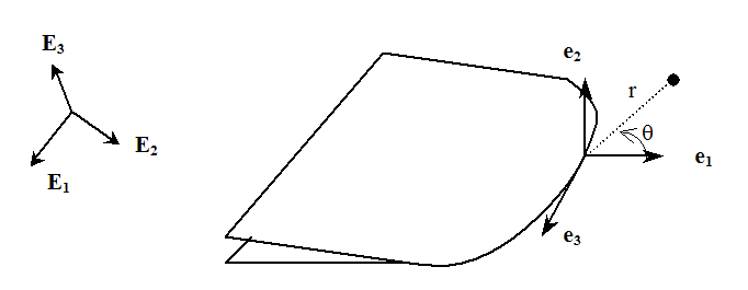
Figure 5.2.2-1 : Polar coordinates, local base, and global base

Let \(\text{DPODL}\) be the matrix of derivatives of polar coordinates in the local base:

\(\text{DPODL}\mathrm{=}\left[\begin{array}{ccc}\frac{\mathrm{\partial }r}{\mathrm{\partial }x}& \frac{\mathrm{\partial }r}{\mathrm{\partial }y}& \frac{\mathrm{\partial }r}{\mathrm{\partial }z}\\ \frac{\mathrm{\partial }\theta }{\mathrm{\partial }x}& \frac{\mathrm{\partial }\theta }{\mathrm{\partial }y}& \frac{\mathrm{\partial }\theta }{\mathrm{\partial }z}\end{array}\right]\mathrm{=}\left[\begin{array}{ccc}\text{cos}\theta & \text{sin}\theta & 0\\ \mathrm{-}\frac{\text{sin}\theta }{r}& \frac{\text{cos}\theta }{r}& 0\end{array}\right]\)

Let \(u\) be an auxiliary field expressed as a function of the polar coordinates \((r,\theta )\). The derivatives of \(u\) with respect to the variables \((r,\theta )\) are determined analytically. They are written in matrix form:

\(\text{DUDPO}\mathrm{=}\left[\begin{array}{cc}\frac{\mathrm{\partial }{u}_{1}}{\mathrm{\partial }r}& \frac{\mathrm{\partial }{u}_{1}}{\mathrm{\partial }\theta }\\ \frac{\mathrm{\partial }{u}_{2}}{\mathrm{\partial }r}& \frac{\mathrm{\partial }{u}_{2}}{\mathrm{\partial }\theta }\\ \frac{\mathrm{\partial }{u}_{3}}{\mathrm{\partial }r}& \frac{\mathrm{\partial }{u}_{3}}{\mathrm{\partial }\theta }\end{array}\right]\)

Then, we write the derivatives in the local base \(({e}_{1},{e}_{2},{e}_{3})\):

\(\text{DUDL}\mathrm{=}\left[\begin{array}{ccc}\frac{\mathrm{\partial }{u}_{1}}{\mathrm{\partial }x}& \frac{\mathrm{\partial }{u}_{1}}{\mathrm{\partial }y}& \frac{\mathrm{\partial }{u}_{1}}{\mathrm{\partial }z}\\ \frac{\mathrm{\partial }{u}_{2}}{\mathrm{\partial }x}& \frac{\mathrm{\partial }{u}_{2}}{\mathrm{\partial }y}& \frac{\mathrm{\partial }{u}_{2}}{\mathrm{\partial }z}\\ \frac{\mathrm{\partial }{u}_{3}}{\mathrm{\partial }x}& \frac{\mathrm{\partial }{u}_{3}}{\mathrm{\partial }y}& \frac{\mathrm{\partial }{u}_{3}}{\mathrm{\partial }z}\end{array}\right]\mathrm{=}\text{DUDPO}\text{.}\text{DPODL}\mathrm{=}\left[\begin{array}{cc}\frac{\mathrm{\partial }{u}_{1}}{\mathrm{\partial }r}& \frac{\mathrm{\partial }{u}_{1}}{\mathrm{\partial }\theta }\\ \frac{\mathrm{\partial }{u}_{2}}{\mathrm{\partial }r}& \frac{\mathrm{\partial }{u}_{2}}{\mathrm{\partial }\theta }\\ \frac{\mathrm{\partial }{u}_{3}}{\mathrm{\partial }r}& \frac{\mathrm{\partial }{u}_{3}}{\mathrm{\partial }\theta }\end{array}\right]\text{.}\left[\begin{array}{ccc}\frac{\mathrm{\partial }r}{\mathrm{\partial }x}& \frac{\mathrm{\partial }r}{\mathrm{\partial }y}& \frac{\mathrm{\partial }r}{\mathrm{\partial }z}\\ \frac{\mathrm{\partial }\theta }{\mathrm{\partial }x}& \frac{\mathrm{\partial }\theta }{\mathrm{\partial }y}& \frac{\mathrm{\partial }\theta }{\mathrm{\partial }z}\end{array}\right]\)

Now it remains to write the derivatives of \(u\) in the global \(({E}_{1},{E}_{2},{E}_{3})\) database. For this, we denote \(R\) the matrix of the vectors of the global base written in the local base (passage matrix):

\({R}_{\alpha m}\mathrm{=}({e}_{\alpha }\mathrm{\cdot }{E}_{m})\)

Let i and j be global indices, the \(j\) th derivative of the \(i\) th component of \(u\) is then written:

\({u}_{i,j}\mathrm{=}{(\mathrm{\sum }_{\alpha \mathrm{=}1}^{3}{u}_{\alpha }{R}_{\alpha i})}_{,j}\mathrm{=}\mathrm{\sum }_{\alpha \mathrm{=}1}^{3}({u}_{\alpha ,j}{R}_{\alpha i}+{u}_{\alpha }{R}_{\alpha i,j})\mathrm{=}\mathrm{\sum }_{\alpha \mathrm{=}1}^{3}(\mathrm{\sum }_{\beta \mathrm{=}1}^{3}({u}_{\alpha ,\beta }{R}_{\beta j}){R}_{\alpha i}+{u}_{\alpha }{R}_{\alpha i,j})\)

In this expression, the \({u}_{\alpha ,\beta }\) terms are the components of the \(\text{DUDL}\) matrix. The term \({R}_{\mathrm{\alpha i},j}\) appears to be the curvature of the local base. It can be overlooked if the curvature of the crack bottom is small. In practice, taking it into account hardly changes the results.

5.2.3. Discretizations

As before, we note s the curvilinear abscissa at the bottom of the crack. Calculating the local value of \({K}_{I}\) , \({K}_{\text{II}}\), and \({K}_{\text{III}}\) requires solving the following variational equation for several fields \({\theta }^{i}\):

\(\begin{array}{c}\frac{(1\mathrm{-}{\nu }^{2})}{E}{\mathrm{\int }}_{{\Gamma }_{0}}{K}_{I}(s){\theta }^{i}(s)\mathrm{\cdot }m(s)\text{ds}\mathrm{=}g{(u,{u}_{I}^{S})}_{{\theta }^{i}}\mathrm{\forall }i\mathrm{\in }\mathrm{[}\mathrm{1,}P\mathrm{]}\\ \frac{(1\mathrm{-}{\nu }^{2})}{E}{\mathrm{\int }}_{{\Gamma }_{0}}{K}_{\text{II}}(s){\theta }^{i}(s)\mathrm{\cdot }m(s)\text{ds}\mathrm{=}g{(u,{u}_{\text{II}}^{S})}_{{\theta }^{i}}\mathrm{\forall }i\mathrm{\in }\mathrm{[}\mathrm{1,}P\mathrm{]}\\ \frac{1}{2\mu }{\mathrm{\int }}_{{\Gamma }_{0}}{K}_{\text{III}}(s){\theta }^{i}(s)\mathrm{\cdot }m(s)\text{ds}\mathrm{=}g{(u,{u}_{\text{III}}^{S})}_{{\theta }^{i}}\mathrm{\forall }i\mathrm{\in }\mathrm{[}\mathrm{1,}P\mathrm{]}\end{array}\) eq. 5.2.3-1

The scalar fields \({K}_{\text{I}}(s)\), \({K}_{\text{II}}(s)\) and \({K}_{\text{III}}(s)\) are discretized on the basis denoted by \({({p}_{j}(s))}_{1\le j\le N}\):

\(\begin{array}{ccc}{K}_{I}(s)& \mathrm{=}& \mathrm{\sum }_{j\mathrm{=}1}^{N}{K}_{Ij}{p}_{j}(s)\\ {K}_{\mathit{II}}(s)& \mathrm{=}& \mathrm{\sum }_{j\mathrm{=}1}^{N}{K}_{\mathit{II}j}{p}_{j}(s)\\ {K}_{\mathit{III}}(s)& \mathrm{=}& \mathrm{\sum }_{j\mathrm{=}1}^{N}{K}_{\mathit{III}j}{p}_{j}(s)\end{array}\)

For theta fields, the approximation [eq.] is retained.

As for \(G\), by injecting discretization expressions into the variational equation [eq.], we get the linear system:

\(\begin{array}{cccc}\underset{{\Gamma }_{0}}{\mathrm{\int }}\mathrm{\sum }_{j\mathrm{=}1}^{N}{K}_{Ij}{p}_{j}(s)\mathrm{\sum }_{k\mathrm{=}1}^{M}({\theta }_{k}^{i}{q}_{k}(s))\mathrm{\cdot }m(s)\mathit{ds}& \text{=}& g{(u,{u}_{I}^{S})}_{{\theta }^{i}},& \mathrm{\forall }i\mathrm{\in }\mathrm{[}\mathrm{1,}P\mathrm{]}\\ \underset{{\Gamma }_{0}}{\mathrm{\int }}\mathrm{\sum }_{j\mathrm{=}1}^{N}{K}_{\mathit{II}j}{p}_{j}(s)\mathrm{\sum }_{k\mathrm{=}1}^{M}({\theta }_{k}^{i}{q}_{k}(s))\mathrm{\cdot }m(s)\mathit{ds}& \text{=}& g{(u,{u}_{\mathit{II}}^{S})}_{{\theta }^{i}},& \mathrm{\forall }i\mathrm{\in }\mathrm{[}\mathrm{1,}P\mathrm{]}\\ \underset{{\Gamma }_{0}}{\mathrm{\int }}\mathrm{\sum }_{j\mathrm{=}1}^{N}{K}_{\mathit{III}j}{p}_{j}(s)\mathrm{\sum }_{k\mathrm{=}1}^{M}({\theta }_{k}^{i}{q}_{k}(s))\mathrm{\cdot }m(s)\mathit{ds}& \text{=}& g{(u,{u}_{\mathit{III}}^{S})}_{{\theta }^{i}},& \mathrm{\forall }i\mathrm{\in }\mathrm{[}\mathrm{1,}P\mathrm{]}\end{array}\)

5.3. G-theta method with X- FEM

So far, the G-theta method has been presented as part of the finite element method (MEF). To adapt the G-theta method to the X- FEM framework, there are very few changes that need to be made. The only difference is in the level of numerical integrations, to calculate domain integrals [eq.]. Just as for the integration of the tangent matrices of these second members, the integration is carried out on the sub-elements.