3. Cracking problem with X- FEM

3.1. General problem

In this part, we recall the equations of the general problem of a cracked structure. We consider a crack \({\Gamma }_{c}\) in a domain \(\Omega \in {\Re }^{3}\) delimited by \(\partial \Omega\) of external normal \({n}_{\mathrm{ext}}\). The lips of the crack are noted \({\Gamma }^{1}\) and \({\Gamma }^{2}\) of external normals \({n}^{1}\) and \({n}^{2}\). The constraint and displacement fields are respectively noted \(\sigma\) and \(u\).

Quasi-static loading is imposed on the structure via a density of volume forces \(f\), a density of surface forces \(t\) on \({\Gamma }_{t}\) and a density of surface forces \(g\) on the lips. The solid is embedded on \({\Gamma }_{u}\).

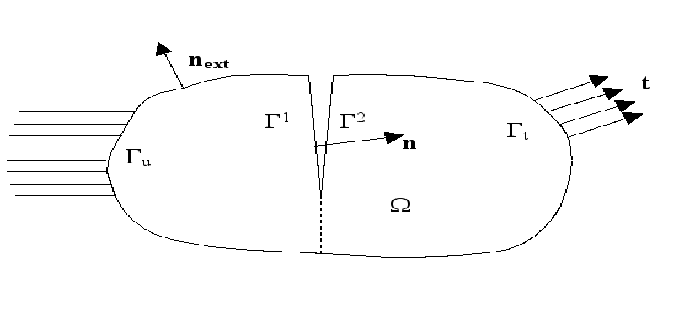
Figure 3.1-1 : General problem notes

The strong form of equilibrium equations and boundary conditions is written as:

\(\begin{array}{}\nabla \cdot \sigma =f\text{dans}\Omega \\ \sigma \cdot {n}_{\mathrm{ext}}=t\text{sur}{\Gamma }_{t}\\ \sigma \cdot {n}^{1}=g\text{sur}{\Gamma }^{1}\\ \sigma \cdot {n}^{2}=g\text{sur}{\Gamma }^{2}\\ u=0\text{sur}{\Gamma }_{u}\end{array}\) eq 3.1-1

We place ourselves in the framework of small deformations and small displacements, for which the deformations-displacements relationship is written:

\(\varepsilon =\varepsilon (u)={\nabla }_{s}u\) eq 3.1-2

where \({\nabla }_{s}\) is the symmetric part of the gradient and \(\varepsilon\) is the strain tensor.

We consider a linear elastic material [1] . The law of behavior of solid \(\Omega\) is written as:

\(\sigma \mathrm{=}C\mathrm{:}\varepsilon \text{dans}\Omega\) eq 3.1-3

where \(C\) is the Hooke tensor.

The principle of virtual work is written as:

\({\int }_{\Omega }\sigma (u):\epsilon (v)d\Omega ={\int }_{\Omega }f\cdot \mathrm{vd}\Omega +{\int }_{{\Gamma }_{t}}t\cdot \mathrm{vd\Gamma }+{\int }_{{\Gamma }_{c}}g\cdot \mathrm{vd\Gamma }\forall v\in {H}_{0}^{1}(\Omega )\) eq 3.1-4

where \({H}_{0}^{1}(O)\) is the Sobolev space of functions whose derivative has an integrable square, cancelling out on \(\partial \mathrm{\Omega }\).

3.2. Enrichment of the displacement approximation

The main idea is to enrich the base of interpolation functions by partitioning the unit [bib 23]. We recall the classical finite element approximation:

\({u}^{h}(x)=\sum _{i\in {N}_{n}(x)}{a}_{i}{\phi }_{i}(x)\)

where \({a}_{i}\) are the degrees of freedom of movement at node i and \({\phi }_{i}\) are the shape functions associated with node i. \({N}_{n}(x)\) is the set of nodes whose support contains the point \(x\). We equate the support of a node i to the support of the shape functions associated with this node, that is to say to the set of points \(x\) such as \({\phi }_{i}(x)\ne 0\).

The enriched approximation is written as:

\({u}^{h}(x)=\sum _{i\in {N}_{n}(x)}{a}_{i}{\mathrm{\varphi }}_{i}(x)+\sum _{j\in {N}_{n}(x)\cap K}{b}_{j}{\mathrm{\varphi }}_{j}(x){H}_{j}\left(\mathit{lsn}(x)\right)+\sum _{k\in {N}_{n}(x)\cap L}\sum _{\mathrm{\alpha }=1}^{4}{c}_{k}^{\mathrm{\alpha }}{\mathrm{\varphi }}_{k}(x){F}^{\mathrm{\alpha }}\left(\mathit{lsn}(x),\mathit{lst}(x)\right)\)

This expression is composed of 3 terms. The 1st term is the classical term continuous. The 2nd and 3rd terms are enriched terms. Being at the heart of the X- FEM method, these terms are explained in the following paragraphs.

3.2.1. Enrichment with a domain selection function (2nd term)

Assume that interface \({\Gamma }_{c}\) partitions the domain such as \(\mathrm{\Omega }={\mathrm{\Omega }}_{\text{+}}\cup {\mathrm{\Omega }}_{\text{-}}\). If \({\Gamma }_{c}\) is a crack, the \(\mathrm{\Omega }\) domain is partitioned in the same way by virtually extending \({\Gamma }_{c}\).

In order to represent the jump in movement through \({\Gamma }_{c}\), we introduce the domain selection function or domain characteristic function \({H}_{j}\left(x\right)\) [bib 76] defined by:

\(\mathit{Si}\phantom{\rule{2em}{0ex}}{x}_{j}\in {\mathrm{\Omega }}_{\text{+}},\phantom{\rule{2em}{0ex}}{H}_{j}(x)=\{\begin{array}{c}\phantom{\rule{2em}{0ex}}0\phantom{\rule{2em}{0ex}}\text{si}\phantom{\rule{0.5em}{0ex}}x\in {\mathrm{\Omega }}_{\text{+}}\\ -2\phantom{\rule{2em}{0ex}}\text{si}\phantom{\rule{0.5em}{0ex}}x\notin {\mathrm{\Omega }}_{\text{+}}\end{array}\)

\(\mathit{Si}\phantom{\rule{2em}{0ex}}{x}_{j}\in {\mathrm{\Omega }}_{\text{-}},\phantom{\rule{2em}{0ex}}{H}_{j}(x)=\{\begin{array}{c}\phantom{\rule{2em}{0ex}}0\phantom{\rule{2em}{0ex}}\text{si}\phantom{\rule{0.5em}{0ex}}x\in {\mathrm{\Omega }}_{\text{-}}\\ +2\phantom{\rule{2em}{0ex}}\text{si}\phantom{\rule{0.5em}{0ex}}x\notin {\mathrm{\Omega }}_{\text{-}}\end{array}\)

Using the normal level set, the quantity \({H}_{j}\left(\text{lsn}\left(x\right)\right)\) is \(0\) if the point \(x\) and the node \({x}_{j}\) are on the same side of the crack and \(\pm 2\) otherwise. The coefficient « 2 » is introduced to have a simpler way of writing the average jump of movement along the interface.

The \({b}_{j}\) are the enriched degrees of freedom. \(K\) is the set of knots whose support is entirely cut by the crack (knots represented by a circle on Figure 3.2.1-1).

Note: for abuse of language, domain selection functions will also be called « Heaviside » functions. But it will be necessary to refer to the definition above, to represent the approximation of the discontinuity of the field of displacement.

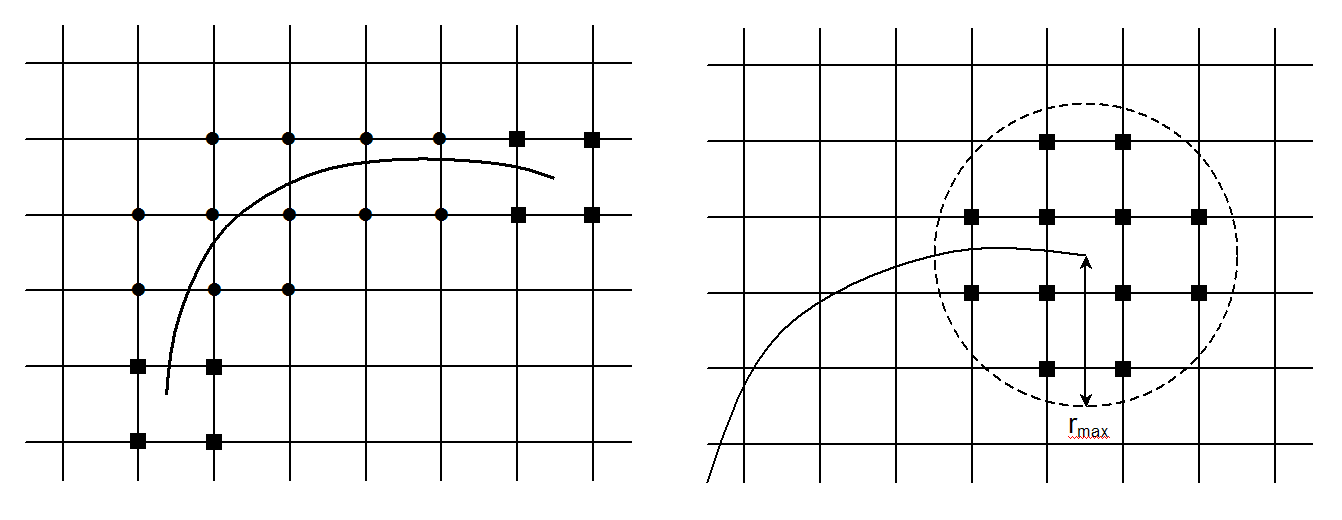
Figure 3.2.1-1: On the left, the « round » nodes are enriched by the Heaviside function and the « square » nodes by the singular functions (topological enrichment). On the right, the « square » nodes are enriched by the singular functions (geometric enrichment).

3.2.2. Enrichment with a domain selection function for a crack branch

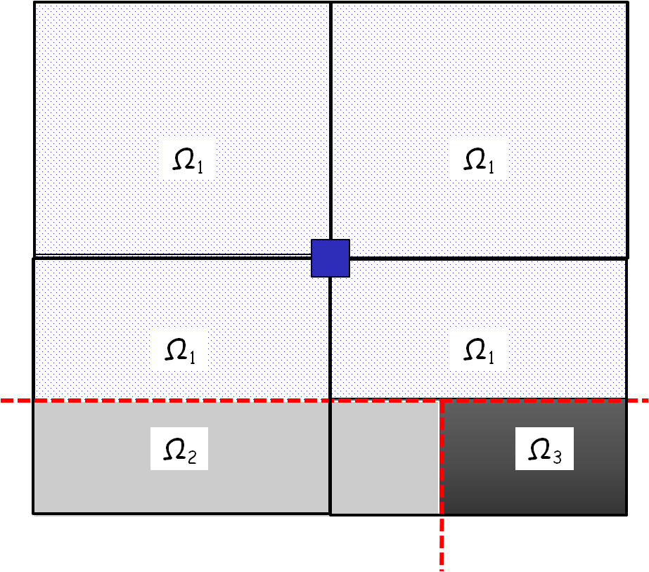
Assume a branch of two discontinuities, which partitions space into three domains such as \(\mathrm{\Omega }={\mathrm{\Omega }}_{\text{1}}\cup {\mathrm{\Omega }}_{\text{2}}\cup {\mathrm{\Omega }}_{\text{3}}\). If it is a branch of two cracks, domain \(\mathrm{\Omega }\) is partitioned in the same way by virtually extending the three crack branches.

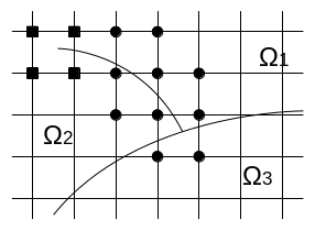
Figure 3.2.2-1partitioning of the domain by a crack junction

For a simple connection, the generalization of domain selection functions leads to the following writing:

\(\begin{array}{c}{u}^{h}(x)=\sum _{i\in {N}_{n}(x)}{a}_{i}{\mathrm{\varphi }}_{i}(x)+\sum _{j\in K\cap {\mathrm{\Omega }}_{\text{1}}}{b}_{j\mathrm{,1}}{\mathrm{\varphi }}_{j}(x){\mathrm{\chi }}_{{\mathrm{\Omega }}_{\text{2}}}+{b}_{j\mathrm{,2}}{\mathrm{\varphi }}_{j}(x){\mathrm{\chi }}_{{\mathrm{\Omega }}_{\text{3}}}\\ +\sum _{j\in K\cap {\mathrm{\Omega }}_{\text{2}}}{b}_{j\mathrm{,1}}{\mathrm{\varphi }}_{j}(x){\mathrm{\chi }}_{{\mathrm{\Omega }}_{\text{1}}}+{b}_{j\mathrm{,2}}{\mathrm{\varphi }}_{j}(x){\mathrm{\chi }}_{{\mathrm{\Omega }}_{\text{3}}}\\ +\sum _{j\in K\cap {\mathrm{\Omega }}_{\text{3}}}{b}_{j\mathrm{,1}}{\mathrm{\varphi }}_{j}(x){\mathrm{\chi }}_{{\mathrm{\Omega }}_{\text{1}}}+{b}_{j\mathrm{,2}}{\mathrm{\varphi }}_{j}(x){\mathrm{\chi }}_{{\mathrm{\Omega }}_{\text{2}}}\end{array}\)

Where \({\mathrm{\chi }}_{{\mathrm{\Omega }}_{\text{i}}}\) are domain selection functions defined by:

\({\mathrm{\chi }}_{{\mathrm{\Omega }}_{\text{i}}}(x)=\{\begin{array}{c}\phantom{\rule{2em}{0ex}}2\phantom{\rule{2em}{0ex}}\text{si}\phantom{\rule{0.5em}{0ex}}x\in {\mathrm{\Omega }}_{\text{i}}\\ \phantom{\rule{2em}{0ex}}0\phantom{\rule{2em}{0ex}}\text{si}\phantom{\rule{0.5em}{0ex}}x\notin {\mathrm{\Omega }}_{\text{i}}\end{array}\)

However, the topological description of the three related domains (Ω1, Ω2, and Ω3) is not trivial, considering the only information provided by the level-sets. Levet-sets make it possible to represent a change in scalar sign through a discontinuity. Whereas we want to represent the partitioning of space in the vicinity of the discontinuity.

From an « elementary » point of view, we note that the sign field of level-sets, read in vector form, corresponds approximately to the partitioning we want to achieve. This partitioning, thanks to the vectorization of scalar level-sets, then makes it possible to reuse the Code_Aster data structures advantageously. However, elementary partitioning alone is insufficient, to represent the « ddl domain » (χ Ωφi).

Note:

In fact, the « ddl domain » corresponds to the collection of partitions of the domain Ω across the entire support of node i. On the support of each node, it is therefore essential to concatenate the elementary partitions corresponding to a given « ddl domain » . This operation is not trivial since sign fields evolve from one element to another (as scalar sign fields are not extended over all elements, to locate the definition of a crack on a few elements of interest, also called « near band » of enrichment). An algorithm dedicated to the concatenation of elementary partitioning has been developed to solve this fundamental difficulty.

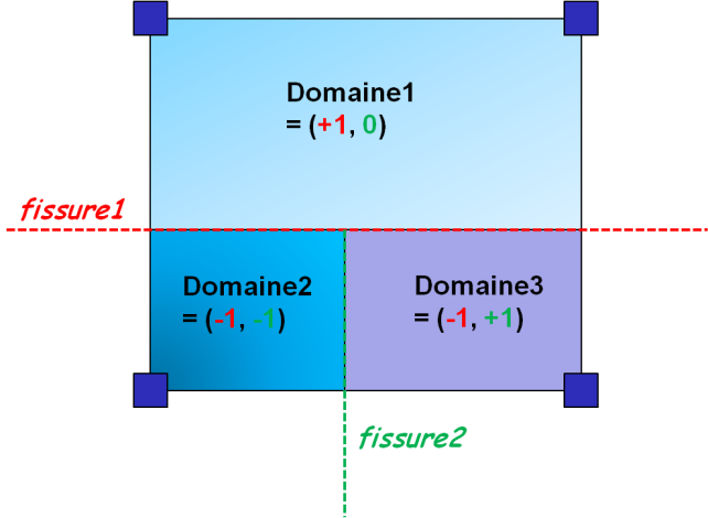
Figure 3.2.2-2: partitioning a multi-cracked element using the « vectorized » sign field. For each domain, the first scalar component of the sign vector corresponds to the characterization of the discontinuity of crack No. 1 and the second scalar component of the sign vector corresponds to the discontinuity of crack No. 2.

Construction of sign functions or junctions:

Recall the construction of Heaviside sign functions or junction-type functions [bib 70]. This is a Heaviside function that is « truncated » at the branch level. The enriched nodes are shown on the.

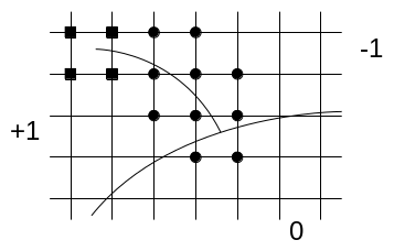
Figure 3.2.2-3: Enrichment for the second crack. Round nodes are enriched by the junction function, which is equal to +1, -1, 0.

The value of this function depends on the normal set levels of the 2 cracks. We consider the sign of the normal level set of crack 1, on the side where crack 2 is defined \(\mathrm{sign}({\mathrm{lsn}}_{1}({\mathrm{fiss}}_{2}))\) (in practice, we look at the sign of a point belonging to the domain of \({\mathrm{lsn}}_{1}\) in which crack 2 is located, cf. operand JONCTION from doc [U4.82.08]). We then have the junction enrichment function for crack 2 which is written as:

\({J}_{2}(x)=\{\begin{array}{}H({\mathrm{lsn}}_{2}(x))\text{si}\mathrm{sign}({\mathrm{lsn}}_{1}({\mathrm{fiss}}_{2}))H({\mathrm{lsn}}_{1}(x))\ge 0\\ 0\text{sinon}\end{array}\)

It is possible to connect a third crack to the first one (for example to model an intersection):

\({J}_{3}(x)=\{\begin{array}{}H({\mathrm{lsn}}_{3}(x))\text{si}\mathrm{sign}({\mathrm{lsn}}_{1}({\mathrm{fiss}}_{3}))H({\mathrm{lsn}}_{1}(x))\ge 0\\ 0\text{sinon}\end{array}\)

If we want to connect the third crack to the second, we must take into account the domain of definition of the first, we will therefore have:

\({J}_{3}(x)=\{\begin{array}{}H({\mathrm{lsn}}_{3}(x))\text{si}\forall i\in [\mathrm{1,2}],\mathrm{sign}({\mathrm{lsn}}_{i}({\mathrm{fiss}}_{3}))H({\mathrm{lsn}}_{i}(x))\ge 0\\ 0\text{sinon}\end{array}\)

If we generalize the approach to a crack \(N\) that connects to the cracks in a set \(K\), we then define the set of cracks \(P\), which contains both all the cracks in \(K\) and all the cracks into which the cracks in \(K\) possibly branch. The junction function is then written in general terms:

\({J}_{N}(x)=\{\begin{array}{}H({\mathrm{lsn}}_{N}(x))\text{si}\forall i\in P,\mathrm{sign}({\mathrm{lsn}}_{i}({\mathrm{fiss}}_{n}))H({\mathrm{lsn}}_{i}(x))\ge 0\\ 0\text{sinon}\end{array}\)

An example of configuration is shown. On this example a crack connectivity tree is constructed. We deduce from this tree that for \(N=3\), we have \(K=2\) and \(P=[\mathrm{1,2}]\). Similarly for \(N=5\), \(K=[\mathrm{3,4}]\) and \(P=[\mathrm{1,2}\mathrm{,3}\mathrm{,4}]\) are deduced. So we have \({J}_{5}(x)=H({\mathrm{lsn}}_{5}(x))\) on the shaded domain of the figure, and zero elsewhere.

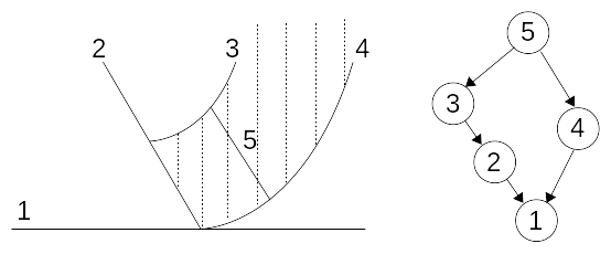
Figure 3.2.2-4: Network of cracks on the left, hierarchy tree on the right, the shaded area corresponds to the domain where the enrichment function of crack 5 is not zero.

Exploitation of sign functions for the assembly of ddls domains:

To build the ddls domains defined in the previous paragraph, we propose to reuse the information from the Heaviside sign field to define elementary partitioning. Since the algorithm is much too complex to explain in terms of data structures, we give a graphical translation of the algorithm. For example, here are the concatenated Heaviside sign fields that we want to use to build elementary partitioning:

Simple crack	Simple junction	Multiple junction

Since the case of a mono-crack is quite easy, we will focus in detail on the case of a simple junction. In the following graphical explanation, we propose to change the perspective from the basic description suggested above. The algorithm will be described from the point of view of node support, which is more suitable for describing nodal enrichment functions.

From the point of view of the node, the information on the sign fields is richer than the idyllic case described above. In fact, the node sees information on nearby cracks, that is to say, located in the first and second bands of elements adjacent to the support of the node. In the node support, there is therefore a crack status (cf. [D4.10.02]) to discriminate cracks intersecting the node support and nearby cracks that do not intersect the node support.

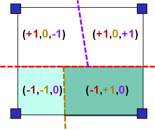
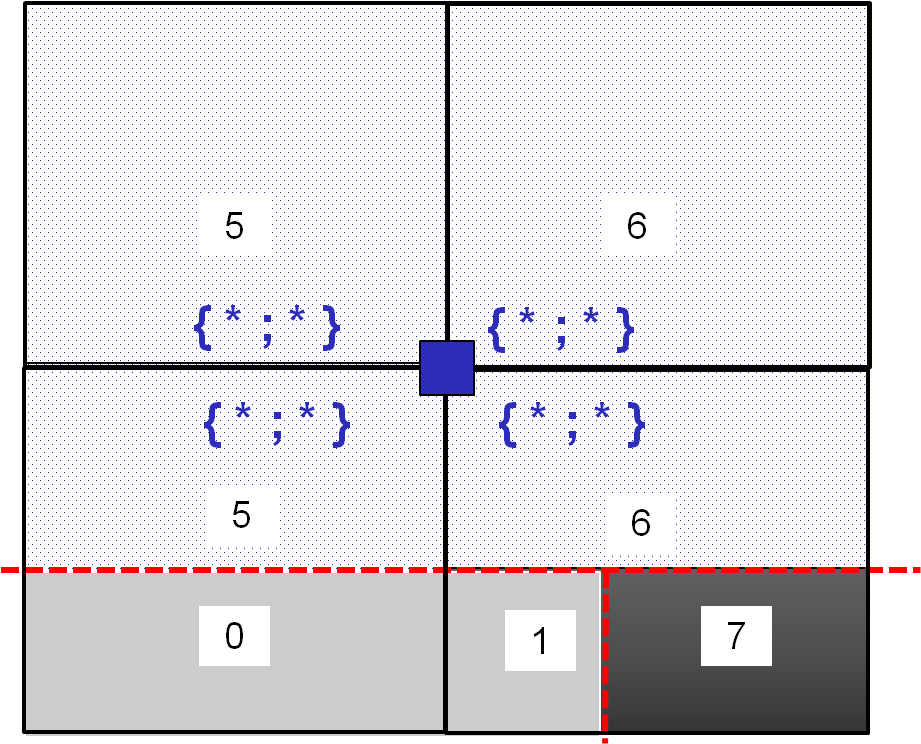
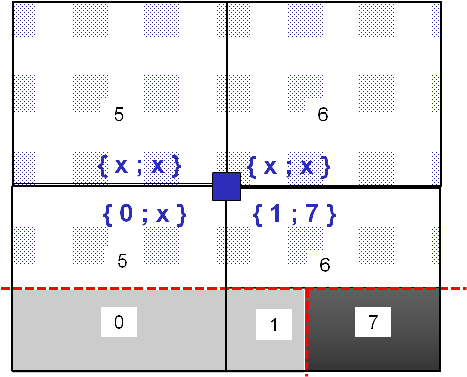
This difficulty makes the association between sign fields and domain partitions non-trivial. This association is necessarily local and must take into account the pollution of sign fields linked to the nearby bands mentioned above. On the example given in the table below, the domains must be associated with the sign field in the following way:

• we associate the domain \({\mathrm{\Omega }}_{\text{1}}\) ↔ with the sign field \(\{\text{+1},\text{0},\text{*}\}\)

• we associate the domain \({\mathrm{\Omega }}_{\text{2}}\) ↔ with the sign field \(\{\text{-1},\text{-1},\text{*}\}\)

• we associate the domain \({\mathrm{\Omega }}_{\text{3}}\) ↔ with the sign field \(\{\text{-1},\text{+1},\text{*}\}\)

Domain partitioning	Associated sign field

To compress the information of the sign vectors, it is preferable to transform the sign vectors using the following reversible coding function:

\(\mathit{code}(\underline{P})=\sum _{\mathit{ifiss}=1}^{\mathit{nfiss}}{3}^{\mathit{nfiss}-\mathit{ifiss}}\left(\mathit{He}(\underline{P},\mathit{ifiss})+1\right)\)

where,

• ifiss is the number in the vector sign field,

• P designates the current point (a node or a gauss point),

• nfiss is the length of the sign field.

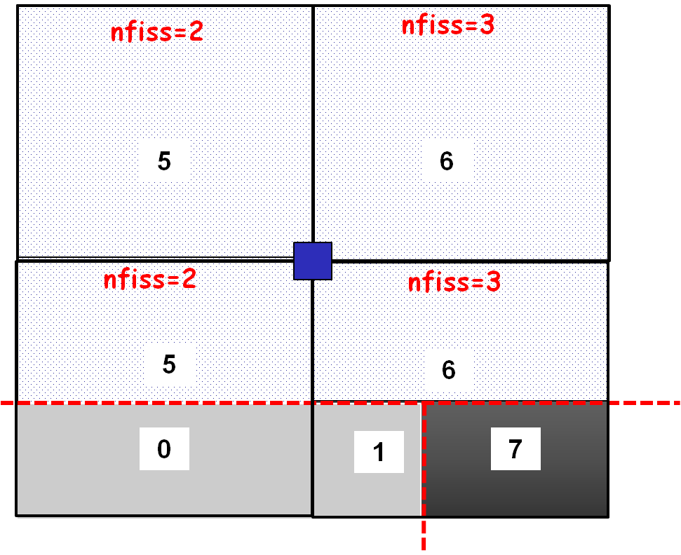
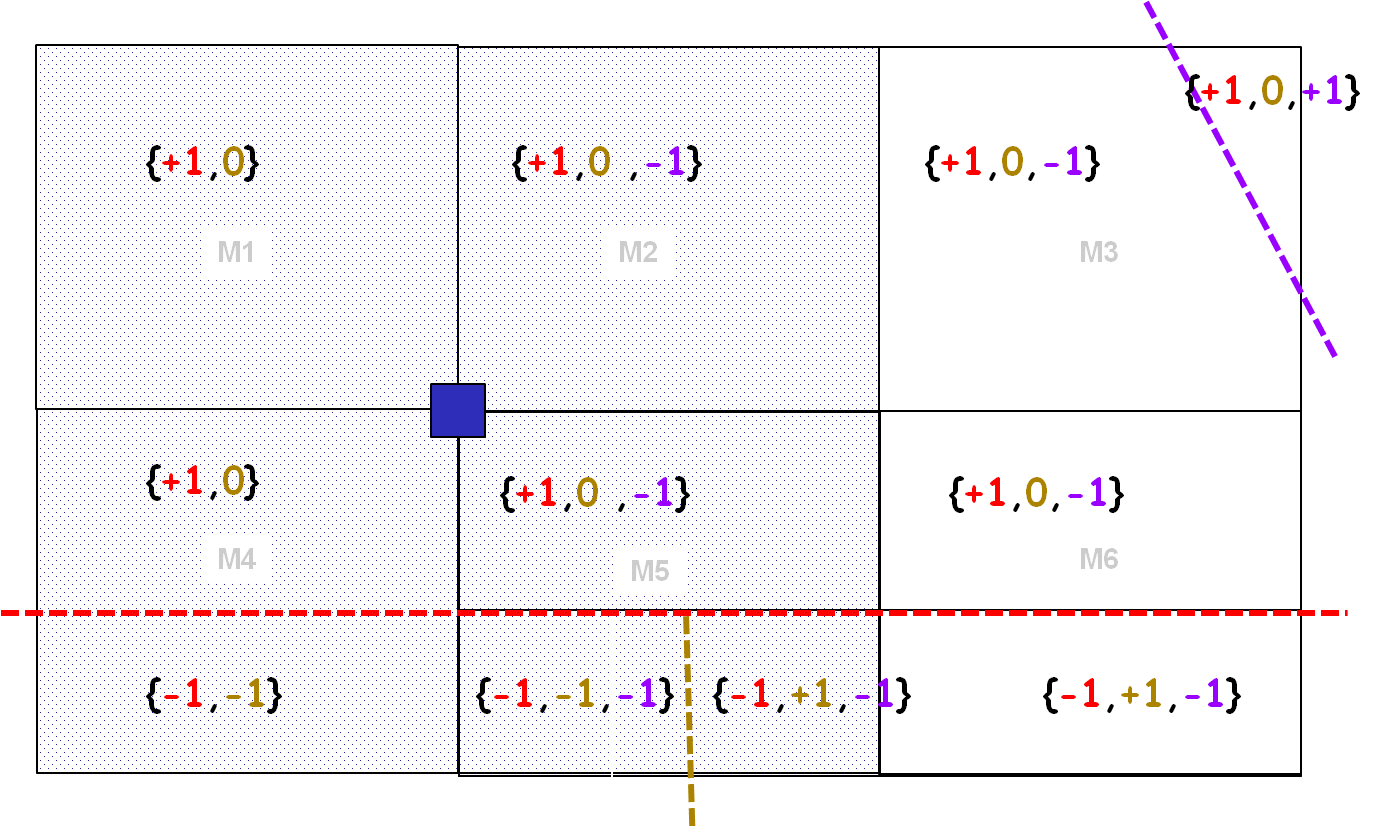
Figure 3.2.2-5: Sign vectors have varying lengths, which leads to different identifiers for the same domain. These identifiers then constitute a second level of sub-partitioning.

Given the variability in the nfiss length of the sign vectors, a domain may have a code that is different from one element to another, as illustrated. For example, domain \({\mathrm{\Omega }}_{\text{1}}\) has two identifiers (5 and 6). These identifiers can be thought of as two*subpartitions* of domain \({\mathrm{\Omega }}_{\text{1}}\).

This sub-partitioning is not a problem as long as the information on this sub-partitioning is grouped at the node level, for the assembly of domain « ddls ». To identify these two ddls domains in each element, all you have to do is concatenate the information on the sub-partitions:

• If a sub-partition of the complementary domain is found, the information is stored in the dedicated location (data structure by node and by element),

• Otherwise, there is no sub-partition for this item.

The result of such an elementary loop is summarized in the table below. In each element we look for a sub-partition of each domain complementary to the blue node. If no sub-partition is found in the element, a cross” x “(or -1 for example) is marked in the dedicated location.

For the blue node belonging to domain \({\mathrm{\Omega }}_{\text{1}}\), the evaluation of the characteristic functions \({\chi }_{{\Omega }_{\text{2}}}\) or \({\mathrm{\chi }}_{{\mathrm{\Omega }}_{\text{3}}}\) is obvious given the partitioning information in the table above. In each element, the first component (of the concatenated field) provides information on the identifier of the first ddl domain \({\mathrm{\chi }}_{{\mathrm{\Omega }}_{\text{2}}}\), the second component (of the concatenated field) provides information on the identifier of the second ddl domain \({\mathrm{\chi }}_{{\mathrm{\Omega }}_{\text{3}}}\):

• If the identifier of the domain to which the Gauss point belongs corresponds to the \(k\in [\mathrm{1,2}]\) component stored at the node, then the characteristic function associated with the \(k\) component takes the value « +2 ». Let us specify again that the component \(k=1\) is associated with the ddl domain \({\mathrm{\chi }}_{{\mathrm{\Omega }}_{\text{2}}}\) and the component \(k=2\) is associated with the ddl domain \({\mathrm{\chi }}_{{\mathrm{\Omega }}_{\text{3}}}\). It is important to note that this position does not change from one element to another, to ensure contiguity of the partitioning. For example, let’s say the collection of identifiers {0.1} corresponding to domain \({\mathrm{\Omega }}_{\text{2}}\). This is exactly the information that is stored in the first position in the data structure at the « blue » node, in the elements intersecting domain \({\mathrm{\Omega }}_{\text{2}}\).

• Otherwise, the characteristic function takes the value zero if the identifier at the Gauss point does not correspond to the component at the node in the element in question.

Notes:

1. Note that the ddl domain \({\chi }_{{\Omega }_{\text{1}}}\) is not treated in the example above. In fact, to represent the two discontinuities introduced by the connection of two cracks, it is necessary to enrich the nodes whose support is intersected by the double discontinuity with two discontinuous functions. We then choose to enrich with the ddls associated with the domains complementary to the domain to which the node*belongs. This choice is well suited, taking into account the packaging problems detailed in §* 3.2.6 .

2. In Code_Aster, we prefer to store Heaviside sign information and domain identifier information at the Gauss point in integration sub-elements.

3.2.3. Enrichment with singular functions (3rd term)

In order to represent the singularity at the bottom of a crack, we enrich the approximation with functions based on the asymptotic developments of the displacement field in linear elastic fracture mechanics [bib 25]. These expressions have been determined for a plane crack in an infinite medium.

\(\begin{array}{}{u}_{1}=\frac{1}{2\mu }\sqrt{\frac{r}{2\pi }}({K}_{1}\text{cos}\frac{\theta }{2}(\kappa -\text{cos}\theta )+{K}_{2}\text{sin}\frac{\theta }{2}(\kappa +2+\text{cos}\theta ))\\ {u}_{2}=\frac{1}{2\mu }\sqrt{\frac{r}{2\pi }}({K}_{1}\text{sin}\frac{\theta }{2}(\kappa -\text{cos}\theta )+{K}_{2}\text{cos}\frac{\theta }{2}(\kappa -2+\text{cos}\theta ))\\ {u}_{3}=\frac{1}{2\mu }\sqrt{\frac{r}{2\pi }}{K}_{3}\text{sin}\frac{\theta }{2}\\ \mu =\frac{E}{2(1+\nu )}\text{et}\kappa =3-4\nu \text{en}\text{déformations}\text{planes}\text{.}\end{array}\) eq. 3.2.3-1

The hypothesis of plane stresses cannot be retained because no cracked plate is in a situation of plane stresses in the vicinity of the singularity, when one places oneself at a finite distance from the skin of the shell.

The basis for describing these fields includes 4 functions:

\(\left\{\sqrt{r}\text{cos}\frac{\theta }{2},\sqrt{r}\text{cos}\frac{\theta }{2}\text{cos}\theta ,\sqrt{r}\text{sin}\frac{\theta }{2},\sqrt{r}\text{sin}\frac{\theta }{2}\text{cos}\theta \right\}\).

Like:

\(\{\begin{array}{c}\text{cos}\frac{\theta }{2}\text{cos}\theta =-\text{sin}\theta \text{sin}\frac{\theta }{2}+\text{cos}\frac{\theta }{2}\\ \text{sin}\frac{\theta }{2}\text{cos}\theta =\text{sin}\theta \text{cos}\frac{\theta }{2}-\text{sin}\frac{\theta }{2}\end{array}\)

3.2.3.1. we then choose the following base [2]

\(F=\left\{\sqrt{r}\text{sin}\frac{\theta }{2},\sqrt{r}\text{cos}\frac{\theta }{2},\sqrt{r}\text{sin}\frac{\theta }{2}\text{sin}\theta ,\sqrt{r}\text{cos}\frac{\theta }{2}\text{sin}\theta \right\}\).

where \((r,\theta )\) are the polar coordinates in the local base at the bottom of the crack (see Figure 2.3-1 and Figure 3.2.3-1).

These coordinates can be easily expressed using level sets, since:

\(r=\sqrt{\text{lsn}\mathrm{²}+\text{lst}\mathrm{²}},\theta =\text{arctan}(\frac{\text{lsn}}{\text{lst}}),\theta \in \left[-\frac{\pi }{2},\frac{\pi }{2}\right]\)

In practice, we use the computer function \(\text{atan2}(\text{lsn},\text{lst})\) instead, which returns the main value of the argument of the complex number \((\text{lst},\text{lsn})\) expressed in radians in the interval \(\left[-\pi ,\pi \right]\).

For points located exactly on the lower lip \((\text{lsn}=0)\), the \(\text{atan2}(\mathrm{0,}\text{lst})\) function gives an angle equal to \(\pi\). In theory, \(\text{atan2}(-\mathrm{0,}\text{lst})\) makes it possible to get \(-\pi\) as expected, but numerically this is not always the case. To overcome this drawback, the following expression is instead used for angle \(\theta\):

\(\theta =H(\text{lsn})\mid \text{atan}2(\text{lsn},\text{lst})\mid ,\theta \in \left[-\pi ,\pi \right]\)

where \(H(\text{lsn})\) is the Heaviside function value. Thus, when one is on the lower lip, the value \(-\pi\) is reached.

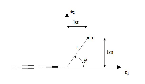
Figure 3.2.3-1 : Polar coordinates in the local base

It should be noted that only the first function of the base is discontinuous across the crack. The other features are only added to improve accuracy. These functions are Westergaard solutions, asymptotic analytical solutions to a 2D elastic fracture problem. This base is well suited to 3D cases [bib 16] [bib 18], at least for cracks whose background is fairly regular. These functions are called « singular » because their derivatives are singular in \(r=0\).

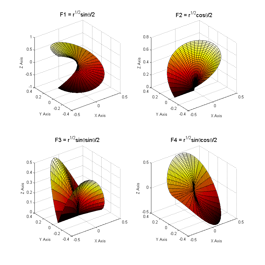
Figure 3.2.3-2 : Enrichment functions at the bottom of the crack

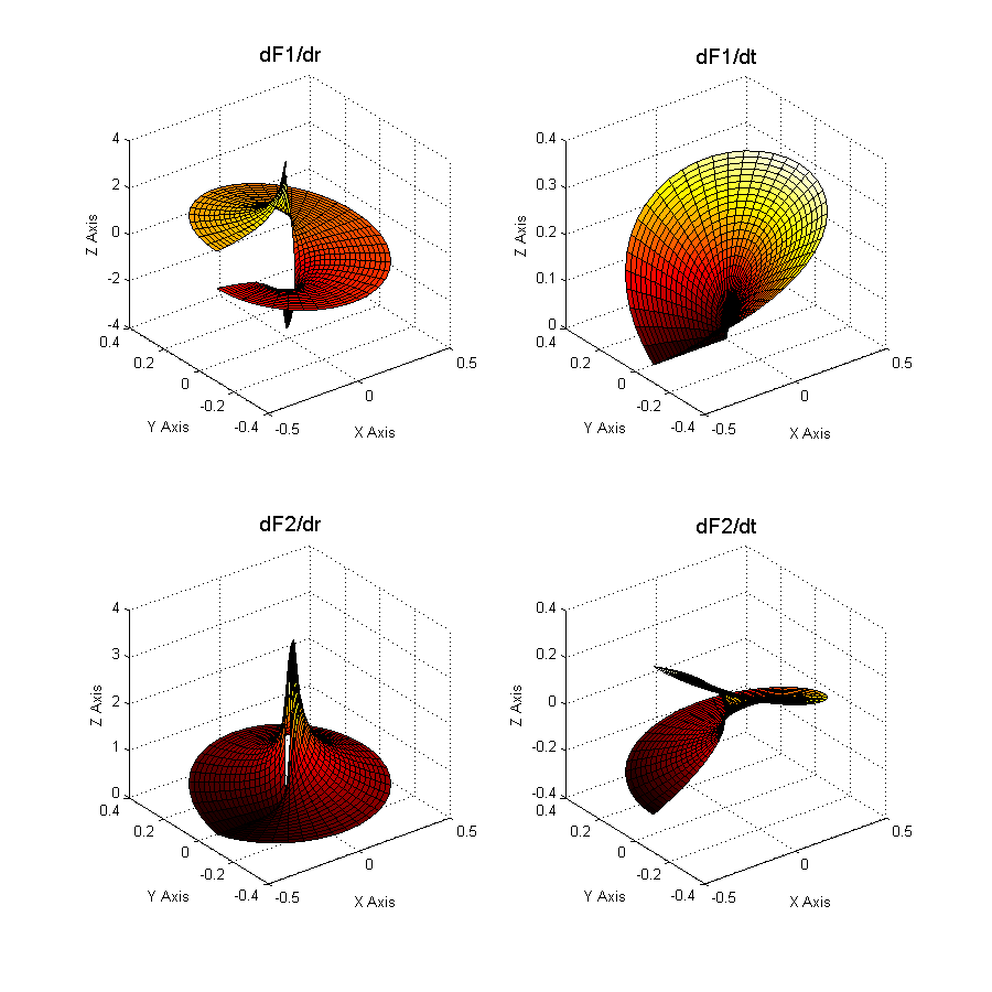
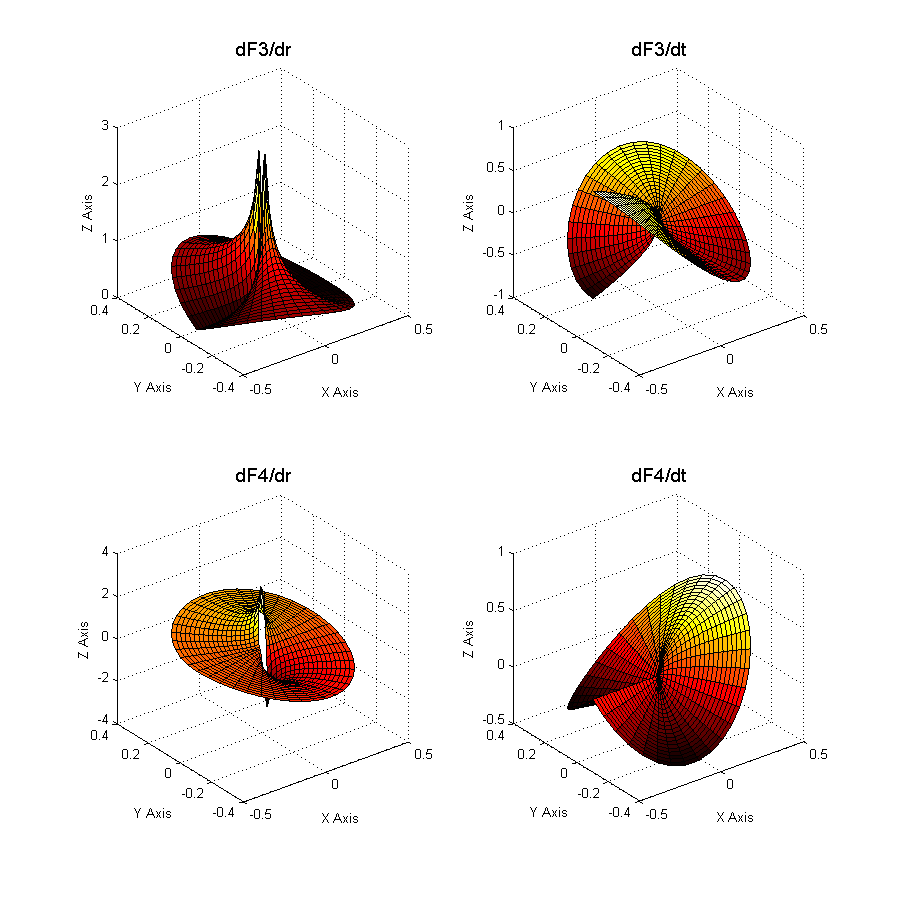
Figure 3.2.3-3 : Derivatives of enrichment functions

The \({c}_{k}^{\alpha }\) are the enriched degrees of freedom. \(L\) is the set of nodes whose support is partially cut by the crack bottom (knots represented by a square on Figure 3.2.1-1). This means that a single layer of elements is enriched around the crack bottom. This enrichment is called « topological ».

3.2.4. Geometric enrichment

From the first papers on X- FEM [bib 24], it was notified that a geometric criterion \({r}_{\text{max}}\) can be defined to determine the nodes enriched by singular functions (see Figure 3.2.1-1):

\(L\mathrm{=}\left\{\text{noeuds}\text{tels}\text{que}r<{r}_{\text{max}}\right\}\)

The first convergence studies were carried out in 2000 as part of GFEM [bib 26], taking into account several layers of elements enriched at the bottom of the crack.

When studying convergence, we are interested in the evolution of the error in relation to the degree of refinement of the mesh. Generally, \(h\) designates a characteristic length of the elements of the mesh, and the aim is to determine the parameter \(\alpha\) called convergence rate (or speed or order), such that the relative error \({e}_{\text{rel}}\) is written in the form:

\({e}_{\mathrm{rel}}={\parallel u-{u}_{h}\parallel }_{{H}^{1}}\underset{h\to 0}{\approx }{\mathrm{Ch}}^{\alpha }\)

where \(C\) is a constant that is independent of \(h\).

Since

\(\text{log}{e}_{\text{rel}}\mathrm{\approx }\text{log}C+\alpha \text{log}h\)

the parameter \(\alpha\) appears as the slope of the line \(\text{log}{e}_{\text{rel}}\) as a function of \(\text{log}h\) when \(h\) tends to 0.

Stazi et al. [bib 27] studies the convergence of the error in energy for an infinite plate with a right crack, in mode I, for linear and quadratic formulations. He notes that the quadratic improves the error, but not the convergence rate. Béchet et al. [bib 28] confirms this observation and shows that a fixed enrichment zone makes it possible to find an almost optimal convergence rate.

At the same time, Laborde*et al.* [bib 29] deepens the question, and tests convergence rates for higher-order polynomial formulations. In addition, it brings improvements in order to regain an optimal rate, or even a superconvergence. The Tableau 3.2.4-1 brings together the results obtained by Laborde for different variants of X- FEM, and this for polynomial approximations of degree \(k=\mathrm{1,2}\mathrm{,3}\).

	FEM	X- FEM	X-	X- FEM (f. a. )	X- FEM (d.g. )	X- FEM (p.m.)
P1	0.5	0.5	0.5	0.5	0.5	1.1
P2	0.5	0.5	0.5	1.8	1.5	2.2
P3	0.5	0.5	0.5	2.6	3.3

Table 3.2.4-1 : Order of convergence of the different variants of X- FEM

The first column corresponds to the orders of convergence of the classical finite element method for a cracking problem. Given the singularity, the convergence speed is in \(\sqrt{h}\) regardless of the \(k\) degree. The 2D simulations carried out on a test problem: rectilinear crack on a square in opening mode I show that X- FEM does not improve the convergence rate. This can be explained by the fact that topological enrichment only concerns a single layer of elements at the bottom of the crack. The area of influence of this enrichment is therefore strongly linked to \(h\). Thus, when \(h\) tends to 0, the size of the enrichment’s area of influence also tends to 0. The idea that seems natural is then to no longer limit the enrichment zone to a single layer of elements, but to expand it to an area of fixed size, independent of the refinement of the mesh. The 3rd column of Tableau 3.2.4-1 shows the results obtained with this method called X- FEM f. a. (for Fixed Enrichment Area). We are almost back to the expected convergence rates (\(\alpha =k\) for an approximation \(\mathit{Pk}\)). However, the packaging is degraded compared to the usual X- FEM method. In order to regain acceptable conditioning, Laborde proposes to bring together the degrees of freedom enriched by the singular functions. Clearly, instead of having different rich ddls for each enriched node, they are globalized in order to have only one for each singular function and per crack (but in 3D, you can’t see how it works in 3D). With this arrangement, conditioning is greatly improved, but convergence rates are lower (X- FEM d. g.). The problem comes from the transition elements between the enriched zone and the non-enriched zone. According to Laborde, the phenomenon is explained by the effect of the partition of the unit that cannot be used on these partially enriched elements. To overcome this defect, an ultimate version is proposed: X- FEM p.m. (for Pointwise Matching). The movements of the nodes on the border between the enriched zone and the non-enriched zone are imposed equal. Thanks to this integration, we obtain expected convergence rates (or even a slight super-convergence).

Note:

For polynomial approximations of degree \(k=\mathrm{2,3}\), Laborde et al. [bib 29 ] like many others use degree form functions \(k\) for classical terms and enriched by discontinuity functions (2nd term), so that the jump is of degree \(k\) . On the other hand, for the terms enriched by the singular functions (3rd term), it is sufficient to use the linear form functions to capture the singularity at the bottom of the crack and not to excessively deteriorate the conditioning of the matrices.

Currently, in Code_Aster, only a degree 1 approximation is possible, and the fact of entering or not entering a radius value for the enrichment zone (keyword RAYON_ENRI) makes it possible to place ourselves respectively in the X- FEM (f. a.) or X- FEM classical frame.

3.2.5. Enrichment in Code_Aster

To find out if a node is enriched by the Heaviside function (« Heaviside » node) or by the singular functions (« crack-tip » node), we calculate the min and the max of the normal level set on all the nodes belonging to the node’s support (the concept of « support » is defined in paragraph [§ 3.2]), and we calculate the min and max of the tangent level set on all the points belonging to the node’s support (the concept of « support » is defined in paragraph [§]), and we calculate the min and max of the level set tangent on all the points belonging to the node’s support (the concept of « support » is defined in paragraph [§]), and we calculate the min and max of the tangent level set on all the points belonging to the node’s support to the support of the node in question where the normal level set is cancelled.

\(\begin{array}{c}j\in K\iff \left(\underset{x\in {N}_{n}(j)}{\text{min}}(\text{lsn}(x))\underset{x\in {N}_{n}(j)}{\text{max}}(\text{lsn}(x))<0\right)\text{et}\left(\underset{x\in {N}_{n}(j)\cap \text{lsn}(x)=0}{\text{max}}(\text{lst}(x))<0\right)\\ k\in L\iff \left(\underset{x\in {N}_{n}(j)}{\text{min}}(\text{lsn}(x))\underset{x\in {N}_{n}(j)}{\text{max}}(\text{lsn}(x))\le 0\right)\text{et}\left(\underset{x\in {N}_{n}(j)\cap \text{lsn}(x)=0}{\text{min}}(\text{lst}(x))\underset{x\in {N}_{n}(j)\cap \text{lsn}(x)=0}{\text{max}}(\text{lst}(x))\le 0\right)\end{array}\)

Similar ideas appear in [bib 17], but it seems that some scenarios were not taken into account. These expressions are the culmination of the first efforts [bib 30] which aimed to determine the types of enrichment using level sets only. The reader will find the corresponding explanatory figures there.

In the case of geometric enrichment at the bottom of a crack, the criterion for selecting nodes is as follows:

\(k\in L\iff \sqrt{\text{lsn}(x)\mathrm{²}+\text{lst}(x)\mathrm{²}}\le {r}_{\text{max}}\)

Regarding the choice of the value of the enrichment radius, nothing is clearly indicated in the literature. However, it seems that a radius equal to between \(1\mathrm{/}5\) and \(1\mathrm{/}10\) of the length of the crack is a relevant choice.

Recent studies have shown that since geometric enrichment greatly degrades the conditioning of the stiffness matrix, it was necessary to limit it in a restricted area around the bottom of the crack, while waiting for treatment to improve the conditioning. An alternative is proposed, which is halfway between topological and geometric enrichment: an enrichment on \(n\) layers [bib 31]. In this case, we calculate a \({r}_{\mathit{max}}\) (unique for each crack) based on the user data for the number of layers, then we apply the previous formula.

Algorithm for choosing node enrichment:

Let \(\mathit{MAFIS}\) be the set of stitches on which the normal level set is cancelled

• loop on all \(P\) nodes of the mesh

initialization of the max and min of the level sets

Let \(A\) and \(B\) be the two ends of the segment

If \(\text{lsn}\left(A\right)=0\) then

Update \(\text{maxlst}\) and \(\text{minlst}\) with \(\text{lst}(A)\) if necessary

End yes

If \(\text{lsn}(B)=0\) then

Update \(\text{maxlst}\) and \(\text{minlst}\) with \(\text{lst}(B)\) if necessary

End yes

If \(\text{lsn}(A)\text{lsn}(B)<0\) then

• in the case of linear interpolation

\(C=A-\frac{\text{lsn}(A)}{\text{lsn}(B)-\text{lsn}(A)}\left(B-A\right)\) eq. 3.2.5.1-1

• in the case of quadratic interpolation

The coordinate in reference space \(\xi\) of the intersection point \(C\) with the curve \(\text{lsn}=0\) on the edge is determined. Its \(\mathit{lst}\) is then given by:

\(\mathit{lst}(C)=\frac{\mathit{lst}(A)\ast \xi \ast (\xi -1)}{2}+\frac{\mathit{lst}(B)\ast (\xi +1)\ast \xi }{2}-\mathit{lst}(M)\ast (\xi -1)\ast (\xi +1)\)

eq. 3.2.5.1-2

Update \(\text{maxlst}\) and \(\text{minlst}\) with \(\text{lst}(C)\) if necessary.

End yes

Update \(\text{maxlsn}\) and \(\text{minlsn}\) if necessary

If \((\text{minlsn}\text{.}\text{maxlsn}<0)\) and \((\text{maxlst}\mathrm{\le }0)\) then \(P\in K\)

topological enrichment cases

If \((\text{minlsn}\text{.}\text{maxlsn}\mathrm{\le }0)\) and \((\text{minlst}\text{.}\text{maxlst}\mathrm{\le }0)\) then \(P\in L\)

case of geometric enrichment:

If \(\sqrt{\text{lsn}{(P)}^{2}+\text{lst}{(P)}^{2}}\mathrm{\le }{r}_{\text{max}}\) then \(P\mathrm{\in }L\)

• end loop

To obtain the equation [éq. 3.2.5.1‑1], as well as the value of the level set tangent to the point \(C\), we first determine the curvilinear abscissa \(s\) such that

\(C=A+s(B-A)\)

thanks to the fact that the normal level set is cancelled in \(C\), i.e.

\(\text{lsn}(C)\mathrm{=}\text{lsn}(A)+s(\text{lsn}(B)\mathrm{-}\text{lsn}(A))\mathrm{=}0\)

We deduce the expression for point \(C\) as well as the value of the tangent level set in \(C\):

\(\begin{array}{c}\text{lst}\left(C\right)=\text{lst}\left(A\right)+s\left(\text{lst}\left(B\right)-\text{lst}\left(A\right)\right)\\ =\text{lst}\left(A\right)-\frac{\text{lsn}\left(A\right)}{\text{lsn}\left(B\right)-\text{lsn}\left(A\right)}\left(\text{lst}\left(B\right)-\text{lst}\left(A\right)\right)\end{array}\)

To obtain, in the quadratic case, the equation [éq. 3.2.5.1‑2], as well as the value of the level set tangent to the point \(C\), the coordinate in the reference space \(\xi\) of the point \(C\) is determined beforehand

\(\mathit{lsn}\) is interpolated quadratically along the edge. It is therefore a question of solving a polynomial of the second degree:

\(0=\frac{\mathit{lsn}(A)\ast \xi \ast (\xi -1)}{2}+\frac{\mathit{lsn}(B)\ast (\xi +1)\ast \xi }{2}-\mathit{lsn}(M)\ast (\xi -1)\ast (\xi +1)\)

Equation \(\mathit{lsn}=0\) has a unique solution on the edge because \(\text{lsn}(A)\text{lsn}(B)<0\)

Once the coordinate \(\xi\) of the point \(C\) is obtained, we interpolate the \(\mathit{lst}\) of the points \(A\), \(B\) and \(M\) to obtain the \(\mathit{lst}\) of the point \(C\):

\(\mathit{lst}(C)=\frac{\mathit{lst}(A)\ast \xi \ast (\xi -1)}{2}+\frac{\mathit{lst}(B)\ast (\xi +1)\ast \xi }{2}-\mathit{lst}(M)\ast (\xi -1)\ast (\xi +1)\)

Note:

The same node can belong to sets \(K\) and \(L\) .

In Code_Aster, it is necessary to define specific types of finite elements, and in order not to multiply the number of possibilities, the choice was made to define 3 types of finite elements X- FEM: the « Heaviside » elements, the « crack-tip » elements and the mixed « Heaviside and crack-tip » elements.

If the mesh has at least one « Heaviside » type node, then it is a « Heaviside » mesh.

If the mesh has at least one « crack-tip » type node, then it is a « crack-tip » mesh.

If the mesh has at least one « Heaviside » node and at least one « crack-tip » node, or if the mesh contains at least one « Heaviside and crack-tip » node, then it is a « Heaviside and crack-tip » mesh.

Note \(\mathit{GRMAEN1}\) the « Heaviside » mesh, \(\mathit{GRMAEN2}\) the « crack-tip » mesh, and the « Heaviside » mesh and the « crack-tip » mesh. \(\mathit{GRMAEN3}\)

Let’s say mesh \(i\), and \(\text{Ni}\) the set of knots \(j\) of stitch \(i\).

\(\begin{array}{c}\text{si}\left(\exists j\in \text{Ni},\text{tel}\text{que}j\in K\right)\text{alors}i\in \text{GRMAEN}1\\ \text{si}\left(\exists j\in \text{Ni},\text{tel}\text{que}j\in L\right)\text{alors}i\in \text{GRMAEN}2\\ \text{si}\left(\exists (j,k)\in {\text{Ni}}^{2},\text{tels}\text{que}j\in K\text{et}k\in L\right)\text{ou}\left(\exists j\in \text{Ni},\text{tel}\text{que}j\in K\cap L\right)\text{alors}i\in \text{GRMAEN}3\end{array}\)

We note that all the nodes of an element will be affected by the same characteristics and the same enrichment, but this is not necessarily what is wanted. It is therefore necessary to cancel out the degrees of freedom enriched « in excess ».

As we saw in the previous paragraph, a « Heaviside » mesh can only include one « Heaviside » type node, for example, the other nodes of the mesh being conventional nodes that do not require any enrichment. However, these nodes will be affected by the degrees of freedom of the « Heaviside » mesh, and therefore by enriched degrees of freedom. Therefore, it is necessary to cancel these degrees of freedom that were wrongly enriched. Cancellation actually makes it possible to move continuously from an enriched zone to a non-enriched zone and allows two types of elements to coexist (in the sense that they share a common border), one enriched, the other not enriched. The unenriched variable is the same on the common border and the degrees of freedom corresponding to the enrichment are set to zero for the element that is enriched on this same border (but not elsewhere in this same element). This way of doing things avoids having to solve the question of « blending elements », which can be treated in [bib 73].

Several cases occur:

• Heaviside degrees of freedom to be cancelled at the classic knots of a Heaviside or mixed mesh

• degrees of freedom crack-tip to be cancelled at the classic knots of a crack-tip or mixed mesh

• Heaviside degrees of freedom to cancel at the crack-tip nodes of a mixed mesh

• crack-tip degrees of freedom to be cancelled at Heaviside nodes in a mixed mesh.

The technique for cancelling these degrees of freedom is explained in detail in [R5.03.54, §4.4].

3.2.6. Enrichment packaging

Conditioning, noted \({10}^{\delta }\), corresponds to the ratio between the largest and the smallest eigenvalue of a system to be inverted. For a double-precision calculation with a numerical error in \({10}^{\mathrm{-}15}\), the relative error obtained on the calculation is of the order of \({10}^{\mathrm{-}15+\delta }\). We must therefore verify condition \(\delta <9\) to guarantee numerical precision in the order of \({10}^{\mathrm{-}6}\).

Geometric enrichment greatly degrades the conditioning of the stiffness matrix [bib 29], [bib 28]. Béchet et al. [bib 28] propose a technique for orthogonalizing degrees of freedom when calculating elementary stiffness matrices in order to improve the conditioning of the assembled matrix. Laborde et al. [bib 29] explain that the poor conditioning is due to the fact that the chosen enrichment base does not form a free family locally. They therefore propose to put a single degree of freedom for these functions over the entire enrichment zone and to connect the movements to the limit between enriched and non-enriched zones in order to find optimal convergence rates. Moreover, the conditioning problem is such that with quadratic elements it becomes impossible to obtain results, without implementing one of the techniques [bib 29], [bib 28]. Indeed, for these elements, the poor conditioning is due not only to the singular part of the enrichment, but also to Heaviside enrichment, when the crack passes very close to a node. The evolution of the number of packages as the interface approaches the nodes of the mesh is shown in the figure, for linear and quadratic elements respectively. The values in this figure are very approximate. On the one hand, we do not take into account the elements of the neighborhood. On the other hand, these values are obtained in a rough manner. In the case of the cube cut in a corner for example (on the right in the figure), we consider the stiffness of the small cube on the corner of the side  \({10}^{\mathrm{-}\gamma }\) instead of the small tetrahedron at the corner. Finally, the conditioning of a global problem is generally greater than the local conditioning and increases when the mesh is refined. By taking into account all these considerations, in practice, packages of an order of 2 to 4 times greater than those in the figure are obtained.

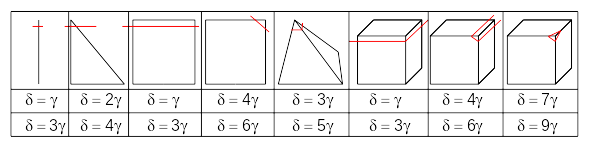
Figure 3.2.6.1-1: the distance to the nearest vertex node normalized by the length of the side equal to \({10}^{\mathrm{-}\gamma }\) we show the dependence of \(\delta\) conditioning number, on the parameter \(\gamma\) for the linear elements in the upper part and quadratic in the lower part.

The technique of readjusting the level set mentioned in paragraph [§ 2.2.4] makes it possible to prevent this poor conditioning. Noting \({10}^{-\gamma }\) the distance from the intersection point of the level set to the nearest vertex node normalized by the length of the side, the adjustment to 1% of the edge length made in paragraph [§ 2.2.4] corresponds to \(\gamma \mathrm{=}2\). This readjustment must act quickly enough so that the conditioning is not too damaged, but not for values of \(\gamma\) that are too low so as not to disturb the system by unrealistically displacing the cracking surface. For quadratic hexahedral elements, if \({10}^{\mathrm{-}15+9\gamma +2}\) must be of the order of \({10}^{\mathrm{-}5}\), we obtain \(9\gamma +2\mathrm{=}10\), which is a readjustment to 13% of the edge length. It is therefore not possible in this case to reasonably activate the readjustment of the level sets at the top, so that the conditioning is not damaged.

Under these conditions, a criterion is set up to detect whether a Heaviside degree of freedom is a problem. If the criterion is met, the degree of freedom is eliminated by zeroing out, as in paragraph [§ 3.2.5.3].

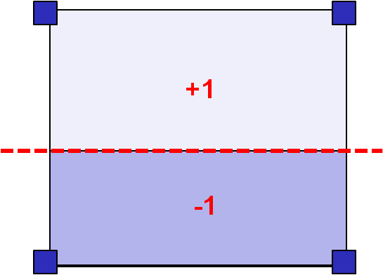
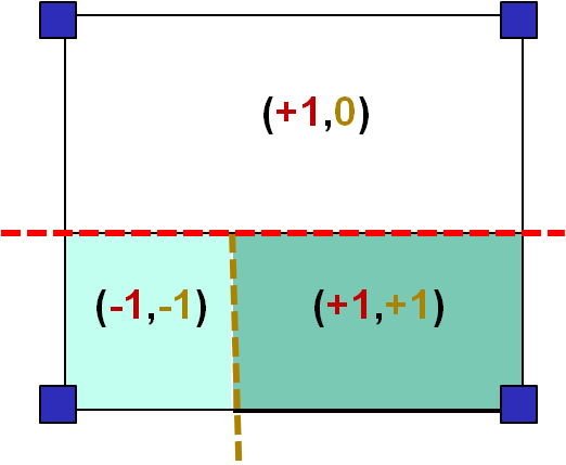
The principle is the same as the volume criterion proposed by Daux [bib 22] for junctions. The idea is to look for each node whose support is cut by the level set, the ratio of the sizes of the zones on both sides of the level set on this support (areas affected by a Heaviside value of ±1). If:

\(\frac{\mathit{min}({V}_{\mathrm{-}1},{V}_{+1})}{{V}_{\mathit{support}}}\mathrm{\le }{10}^{\mathrm{-}\alpha }\) eq, 3.2.6.2-1

the Heaviside degrees of freedom of the node in question are set to zero in all directions.

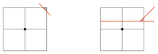
Figure ‑3.2.6.2-1: illustration of the implementation of the volume criterion. The support for the node cut by the level set is shown. We compare the gray and white volumes with respect to the total volume of the node support (meeting of the gray and white volumes) in the case of a crack (left) and a junction (right).

While this criterion is relevant for linear elements (triangles, tetrahedra) with a value of \(\alpha\) of 4, it is not satisfactory for multi-linear elements (quadrangles, pyramids, pentahedra, hexahedra) and quadratic elements. In fact, the value of \(\alpha\) of 4 leads to the elimination of degrees of freedom that should not be eliminated, which disrupts the solution, while higher values of \(\alpha\) degrade the conditioning. In order to take these elements into account, a stiffness criterion is used, which is based on a comparison of the rigidities of the support and no longer simply of the volumes. For each node whose support is cut by the level set, for this support, we look at the ratio of the rigidities of the zones on both sides of the level set (areas affected by a Heaviside value of ±1). If in a \(n\) node where \(\mathit{se}\) are the sub-elements of its support, we have:

\(\frac{\mathit{min}({\mathrm{\sum }}_{{\mathit{se}}_{\mathrm{-}1}}{\mathrm{\int }}_{{\Omega }_{\mathit{se}}}{\mathrm{\parallel }{\phi }_{n,X}\mathrm{\parallel }}^{2}d{\Omega }_{\mathit{se}},{\mathrm{\sum }}_{{\mathit{se}}_{+1}}{\mathrm{\int }}_{{\Omega }_{\mathit{se}}}{\mathrm{\parallel }{\phi }_{n,X}\mathrm{\parallel }}^{2}d{\Omega }_{\mathit{se}})}{{\mathrm{\sum }}_{\mathit{se}}{\mathrm{\int }}_{{\Omega }_{\mathit{se}}}{\mathrm{\parallel }{\phi }_{n,X}\mathrm{\parallel }}^{2}d{\Omega }_{\mathit{se}}}\mathrm{\le }{10}^{\mathrm{-}\delta }\) eq 3.2.6.2-2

where \({\phi }_{n,X}\) is the derivative of the shape function at node \(n\) in the global direction \(X\), then the Heaviside degrees of freedom at node \(n\) are set to zero in all directions. It will be noted that the behavior is not present in the stiffness criterion of eq, the criterion having been standardized. This makes it possible to discriminate in advance the degrees of freedom to be eliminated, without knowing the problem to be solved (non-linearities, plasticity, contact, etc.). This criterion, which is very similar to a conditioning criterion, leads us to choose values of \(\delta\) between 8 and 10. In practice, we take a value of \(\delta\) out of 9.

The criterion described in eq quantifies, in order of magnitude, the compromise between quality of the solution and packaging. As this criterion is only valid in terms of magnitude, it is not necessarily relevant to calculate all the integrals exactly. In Aster programming, we therefore approximate the integral calculation on the sub-elements ([bib 72]):

\({\int }_{{\Omega }_{\mathrm{se}}}{\parallel {\phi }_{n,X}\parallel }^{2}d{\Omega }_{\mathrm{se}}\approx \text{}{\parallel {\phi }_{n,X}({G}^{\mathrm{se}})\parallel }_{\infty }^{2}{V}^{\mathrm{se}}\) eq 3.2.6.2-3

where \({G}^{\mathrm{se}}\) refers to the barycenter of the sub-element, \({V}^{\mathrm{se}}\) the volume of the sub-element.

Instead of calculating the integral on the sub-element, we evaluate the derivatives of form functions at one point. This strategy makes it possible to capture the criterion for eliminating eq in order of magnitude, with a low calculation cost.

This approximation is robust and inexpensive with linear elements.

On the other hand, with quadratic elements, the derivatives of form functions admit roots. The calculation at one point is risky: the barycenter may be a root of the derivatives of form functions, where the estimate will be zero, but the integral on the sub-element will not be. This poor estimate can lead to random eliminates, which disrupts the solution and is not an acceptable step.

We therefore strengthen the estimate for the quadratic elements, by adding other evaluation points, in addition to the barycenter:

\({\int }_{{\Omega }_{\mathrm{se}}}{\parallel {\phi }_{n,X}\parallel }^{2}d{\Omega }_{\mathrm{se}}\approx \text{}{\mathrm{max}}_{{P}_{i}\in {\Omega }_{\mathrm{se}}}({\parallel {\phi }_{n,X}({P}_{i})\parallel }_{\infty }^{2}){V}^{\mathrm{se}}\) eq 3.2.6.2-4

For the evaluation to be relevant, the points are sufficiently well distributed: we consider the points equidistant between the vertex nodes and the barycenter (for example, 3 points for a tri6).

\(\text{{}{P}_{i}\text{}}=\text{{}{G}^{\mathrm{se}}\text{}}\cup \text{{}\frac{{\mathrm{Node}}_{i}+{G}^{\mathrm{se}}}{2}\text{}}\) eq 3.2.6.2-5

However, the following criticisms can be made in relation to these estimated criteria:

• on the one hand, they do not guarantee the control of the packaging just before disposal. As long as the elimination is not performed, the conditioning increases in \({10}^{n\times \gamma }\) (figure), which can lead to the stopping of the direct solver, in an arbitrary manner. This phenomenon is exacerbated with quadratic elements, or even figures.

• on the other hand, an analysis of these various criteria is done in [bib 72]. It shows that the removals lead to an absence of convergence of the energy error on a simple example of homogeneous compression of a cube crossed by an inclined interface. The proposed solution consists in replacing the elimination of Heaviside degrees of freedom by an orthogonalization of the local stiffness matrices, an idea that comes from the preconditioner X- FEM of [bib 28]. In order to overcome this last difficulty, it is necessary to estimate local stiffness matrices at least in triple precision [bib 72].

To address the first criticism, that is to say to stem the exponential increase in conditioning, we have implemented in the Code_Aster, the preconditioner proposed by Béchet et al. [bib 28].

This is an automatic and algebraic procedure, to « orthogonalize » the degrees of freedom associated with a XFEM node. In fact, the enrichment functions XFEM rely on the nodal functions \({\Phi }_{i}\) to describe either the discontinuity of the displacement by the jump functions \(H{\Phi }_{i}\), or the crack background by the singular functions \({F}^{\alpha }{\Phi }_{i}\). The functions introduced by enrichment XFEM are not orthogonal to the shape functions in each node XFEM. In addition, the enrichment functions XFEM and the nodal functions share the same support: there are situations where the functions XFEM are similar to the nodal functions, to the point of becoming almost collinear.

Information on collinearity is carried in stiffness matrix \(K\): stiffness matrix conditioning increases if collinearity increases at least in one XFEM node. From a more formal point of view, the stiffness matrix (cf.§ 3.5.1) derives from the discretization of a positive symmetric bilinear form. So, there is a scalar product \({\langle \mathrm{.},\mathrm{.}\rangle }_{K}\) such that, the term in the stiffness matrix \({K}_{i,x}\) representing the collinearity between the nodal function \({\Phi }_{i}\) and the enrichment function \({F}_{x}{\Phi }_{i}\), can be rewritten:

\({K}_{i,x}={\langle {\Phi }_{i},{F}_{x}{\Phi }_{i}\rangle }_{K}\) eq 3.2.6.3-1

Béchet [bib 28] proposes the construction of a pre-conditioner such as:

\(K\to \stackrel{̃}{K}={P}_{c}^{T}K{P}_{c}\) eq 3.2.6.3-2

The original matrix system is then transformed in the following manner:

\(Ku=f\to \{\begin{array}{c}\stackrel{̃}{K}\stackrel{̃}{u}=\stackrel{̃}{f}\\ \stackrel{̃}{f}={P}_{c}^{T}f\\ u={P}_{c}\stackrel{̃}{u}\end{array}\) eq 3.2.6.3-3

Thus, Béchet [bib 28] builds the new matrix \(\stackrel{̃}{K}\) to respect the following orthogonality condition:

\({\stackrel{̃}{K}}_{i,x}={\langle {\Phi }_{i},{F}_{x}{\Phi }_{i}\rangle }_{\stackrel{̃}{K}}={\langle {P}_{c}{\Phi }_{i},{P}_{c}{F}_{x}{\Phi }_{i}\rangle }_{K}=0\) eq 3.2.6.3-4

In other words, the new functional base \(\left({P}_{c}{\Phi }_{i},{P}_{c}{F}_{x}{\Phi }_{i}\right)\) (through the change of base \({P}_{c}\)) is orthogonal, on the support of each node XFEM. Therefore, the new matrix system to be inverted \(\stackrel{̃}{K}\stackrel{̃}{u}={P}_{c}^{T}f\) is better conditioned regardless of the position of the interface, cf. § 3.2.6.2.

The construction of \(\stackrel{̃}{K}\) is not a unique step. [bib 28] proposes to use the Cholesky factorization of local stiffness matrices, associated with each XFEM node:

\({K}_{\mathit{loc}}^{i}=\left[\begin{array}{ccc}{\langle {\Phi }_{i},{\Phi }_{i}\rangle }_{K}& {\langle {\Phi }_{i},H{\Phi }_{i}\rangle }_{K}& {\langle {\Phi }_{i},{F}^{\alpha }{\Phi }_{i}\rangle }_{K}\\ {\langle {\Phi }_{i},H{\Phi }_{i}\rangle }_{K}& {\langle H{\Phi }_{i},H{\Phi }_{i}\rangle }_{K}& {\langle H{\Phi }_{i},{F}^{\alpha }{\Phi }_{i}\rangle }_{K}\\ {\langle {\Phi }_{i},{F}^{\alpha }{\Phi }_{i}\rangle }_{K}& {\langle H{\Phi }_{i},{F}^{\alpha }{\Phi }_{i}\rangle }_{K}& {\langle {F}^{\alpha }{\Phi }_{i},{F}^{\alpha }{\Phi }_{i}\rangle }_{K}\end{array}\right]\) eq 3.2.6.3-5

The matrix \({K}_{\mathit{loc}}^{i}\) is symmetric definite positive. It therefore admits a factorized Cholesky, that is to say, that there is an upper triangular matrix \({S}_{i}\) such that:

\({K}_{\mathit{loc}}^{i}={S}_{i}^{T}{S}_{i}\) eq 3.2.6.3-6

In an optimal storage configuration contiguous with degrees of freedom, [bib 28] then chooses one diagonal preconditioner per block, such as:

\({P}_{c}=\left[\begin{array}{cccccc}{P}_{c}^{1}& 0& 0& \mathrm{...}& \mathrm{...}& \mathrm{...}\\ 0& {P}_{c}^{2}& 0& \mathrm{...}& 0& \mathrm{...}\\ 0& 0& {P}_{c}^{3}& \mathrm{...}& \mathrm{...}& \mathrm{...}\\ \mathrm{...}& \mathrm{...}& \mathrm{...}& \ddots & \mathrm{...}& \mathrm{...}\\ \mathrm{...}& 0& \mathrm{...}& \mathrm{...}& {P}_{c}^{i}& \mathrm{...}\\ \mathrm{...}& \mathrm{...}& \mathrm{...}& \mathrm{...}& \mathrm{...}& \ddots \end{array}\right]\) eq 3.2.6.3-7

where \({P}_{c}^{i}=\{\begin{array}{c}{S}_{i}^{-1}\text{si}i\text{est un noeud XFEM}\\ {I}_{d}\text{sinon}\end{array}\) eq 3.2.6.3-8

with \({S}_{i}^{-1}\) the inverse of the Cholesky factored matrix. The new stiffness matrix \(\stackrel{̃}{K}\) verifies the support of the XFEM node locally:

\({\stackrel{̃}{K}}_{\mathit{loc}}^{i}={\left({P}_{c}^{i}\right)}^{T}{K}_{\mathit{loc}}^{i}{P}_{c}^{i}={\left({S}_{i}^{-1}\right)}^{T}{K}_{\mathit{loc}}^{i}{S}_{i}^{-1}={\left({S}_{i}^{-1}\right)}^{T}\left({S}_{i}^{T}{S}_{i}\right){S}_{i}^{-1}={I}_{d}\) eq 3.2.6.3-9

\({I}_{d}\) refers to the identity matrix. \({I}_{d}\) therefore respects the orthogonality condition of the equation.

In practice, it is necessary to scale the new \({\stackrel{̃}{K}}_{\mathit{loc}}^{i}\) matrix with the rest of the stiffness matrix. The following preconditioner is therefore preferred to the preconditioner:

\({P}_{c}^{i}=\sqrt{\mathit{scal}}\times {S}_{i}^{-1}\) eq 3.2.6.3-10

where \(\mathit{scal}\) is a scaling coefficient such as: \(\mathit{scal}=\frac{\mathit{max}(∣\mathit{diag}(K)∣)+\mathit{min}(∣\mathit{diag}(K)∣)}{2}\)

Consequently, the new pre-conditioned local matrix complying with the orthogonality condition is:

\({\stackrel{̃}{K}}_{\mathit{loc}}^{i}={\left({P}_{c}^{i}\right)}^{T}{K}_{\mathit{loc}}^{i}{P}_{c}^{i}=\mathit{scal}\times {I}_{d}\) eq 3.2.6.3-11

Moreover, the use of a Cholesky factorization is risky if the conditioning of the local stiffness matrix \({K}_{\mathit{loc}}^{i}\) deteriorates. In case of failure of the Cholesky factorization, we orthogonalize the local matrix using a SVD (decomposition into singular values):

\({K}_{\mathit{loc}}^{i}={U}_{i}{D}_{i}{U}_{i}^{T}\) eq 3.2.6.3-12

where \({U}_{i}\) is an orthogonal matrix and \({D}_{i}\) is a diagonal matrix with strictly positive values.

The following choice of preconditioner is then made alternately:

\({P}_{c}^{i}=\sqrt{\mathit{scal}}\times {U}_{i}\sqrt{{D}_{i}^{-1}}\) eq 3.2.6.3-13

It is easy to verify that this choice makes it possible to respect the orthogonality condition:

\({\stackrel{̃}{K}}_{\mathit{loc}}^{i}={\left({P}_{c}^{i}\right)}^{T}{K}_{\mathit{loc}}^{i}{P}_{c}^{i}={\left(\sqrt{\mathit{scal}}\times {U}_{i}\sqrt{{D}_{i}^{-1}}\right)}^{T}\left({U}_{i}{D}_{i}{U}_{i}^{T}\right)\left(\sqrt{\mathit{scal}}\times {U}_{i}\sqrt{{D}_{i}^{-1}}\right)=\mathit{scal}\times {I}_{d}\)

In summary, the construction of the Béchet preconditioner [bib 28] involves 4 steps:

1. the extraction of local matrices \({K}_{\mathit{loc}}^{i}\) in the stiffness matrix (i.e. block matrices associated with the ddls carried by the nodes XFEM no. \(i\)).

2. the calculation of local pre-conditioning matrices \({P}_{c}^{i}\) (cf. equation or),

3. assembling the pre-conditioner (cf. equation),

4. finally, the transformation of the matrix system (cf. equations and).

Note:

Note that the transformation of the matrix system presents a significant computer difficulty in the code_aster, given the complexity of the data structure for storing matrices (cf. [D4.06.10] and [D4.06.07]).

3.3. Sub-division

Particular attention must be paid when numerically integrating the terms of stiffness and the second member of an element crossed by the crack. In fact, on an element crossed by a crack, the displacement gradients may be discontinuous, and in this case the numerical integration of Gauss-Legendre over the whole of the element is not applicable. In order to return to conventional conditions of regularity, integration should be carried out in areas where the integrand is at least continuous. For an element crossed by a crack, it is therefore necessary to integrate separately on both sides of the crack (this appears for the first time in [bib 24] for 2D and in [bib 32] for 3D). Several procedures are possible, and easily implemented in 2D. The difficulties appear with 3D.

An attempt is made to sub-cut into sub-tetrahedra any volume element (tetrahedron, pentahedron, hexahedron) cut by a surface. It should be noted that this cut is only used for integration purposes, it is purely virtual and no node is added to the mesh. The mesh is not changed in any way.

For pentahedra and hexahedra, the number of possibilities being too large and the configurations too complicated, it is preferable to reduce ourselves to the cutting of tetrahedra. In this way, the large number of cutting possibilities is « condensed » into a few configurations. In other words, we are formulating the « clustering » of a large set (number of intersection configurations) to a small set (reduced number of cutting configurations in a tetrahedron).

In fact, the « condensation » algorithm builds a bijective application, from the parent polyhedron, to some reference cutting configurations. This application can be broken down into two bijective operations:

1 — An (explicit) bijection towards the cutting of a tetrahedron: We therefore carry out a preliminary phase which consists in systematically cutting quadrangles, pyramids, pentahedra and hexahedra into tetrahedra. This bijection is not unique. As can be seen on the, there are two bijections to divide a quadrangle into two triangles (the same for a pyramid), 6 bijections to divide a pentahedron into 3 tetrahedra and 6 bijections to divide a hexahedron into 2 pentahedra which are then divided into tetrahedra. In the case of the hexahedron, each cutting configuration is thus obtained twice. The maximum number of distinct bijections to divide a hexahedron into 6 tetrahedra is therefore \(\frac{{6}^{3}}{2}=108\).

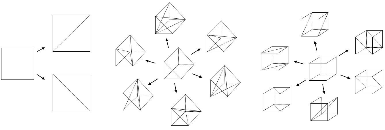
Figure 3.3-1 : Dividing a quadrangle into two triangles (left), dividing a pentahedron into 3 tetrahedra (middle), and dividing a hexahedron into 2 pentahedra (right)

In § 3.3.1 to § 3.3.3, we present the bijection selected by default for the division of non-simplicial elements into tetrahedra (or triangles for the 2D case).

This is a bijection, because we build an (invertible) application that associates the relative numbering of the vertex nodes in a subtetrahedron with the absolute numbering of the nodes in the mesh. The direct application is stored in the connectivity table (see [D4.10.02]: data structures XFEM).

2 — An (implicit) bijection to a reference cutting configuration: on the one hand, we identify the reference cutting configuration corresponding to the tetrahedron to be cut, on the other hand, we « geometrically » return the tetrahedron, to « superimpose » it on this reference cutting configuration (for example). Clearly, the nodes of the subtetrahedron are identified with the nodes of the reference cutting element (this is the direct application of bijection). The multiple cutting possibilities, linked to the different possibilities of ordering the edges and the points of intersection, are then « condensed ».

Subsequently, this operation facilitates the scheduling of the middle nodes of the quadratic subtetrahedra for computer storage. In fact, the ordering of the new middle nodes no longer depends on the faces or edges where they are calculated, but on a single reference cut configuration. Consequently, the new calculated middle nodes are necessarily ordered in the same way, in the reference cut subtetrahedron. Then, these middle nodes are positioned on the edges of the tetrahedron by the reverse application (from the identification of the nodes above). The bijection used is therefore tacit.

The procedures for scheduling and calculating midpoints are explained below.

3.3.1. Preliminary phase of cutting hexahedra to reduce to tetrahedra

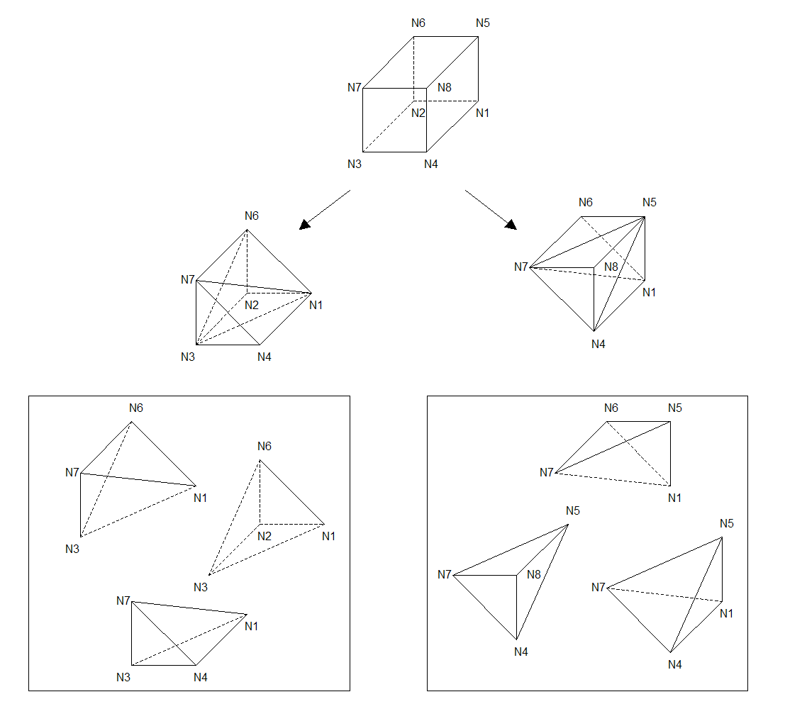
Figure 3.3.1-1 : Division of a hex ahedron (hexa8) into tetrahedra

A hexahedron is then divided into 6 tetrahedra, listed in the following table:

hexahedron	tetrahedron
\(\mathit{N1}\mathit{N2}\mathit{N3}\mathit{N4}\mathit{N5}\mathit{N6}\mathit{N7}\mathit{N8}\)	\(\mathit{N7}\mathit{N4}\mathit{N3}\mathit{N1}\)
	\(\mathit{N1}\mathit{N6}\mathit{N2}\mathit{N3}\)
	\(\mathit{N3}\mathit{N6}\mathit{N7}\mathit{N1}\)
	\(\mathit{N6}\mathit{N1}\mathit{N5}\mathit{N7}\)
	\(\mathit{N4}\mathit{N7}\mathit{N8}\mathit{N5}\)
	\(\mathit{N4}\mathit{N5}\mathit{N1}\mathit{N7}\)

Table 3.3.1-1 : Division of a hexahedron into tetraheders

Note that this division is the choice made by default but we could have chosen another way of cutting a hexahedron into 2 pentahedra as well as another way of cutting a pentahedron into 3 tetrahedra.

If the element is quadratic (HEXA20, PENTA15,…), the same subdivision into tetrahedra is used, as explained above.

In addition, the middle nodes on the new edges generated by the cut must be taken into account: these middle nodes coincide with the middle nodes of the complete element. We therefore virtually add to the element, the middle nodes necessary to find the complete element of.

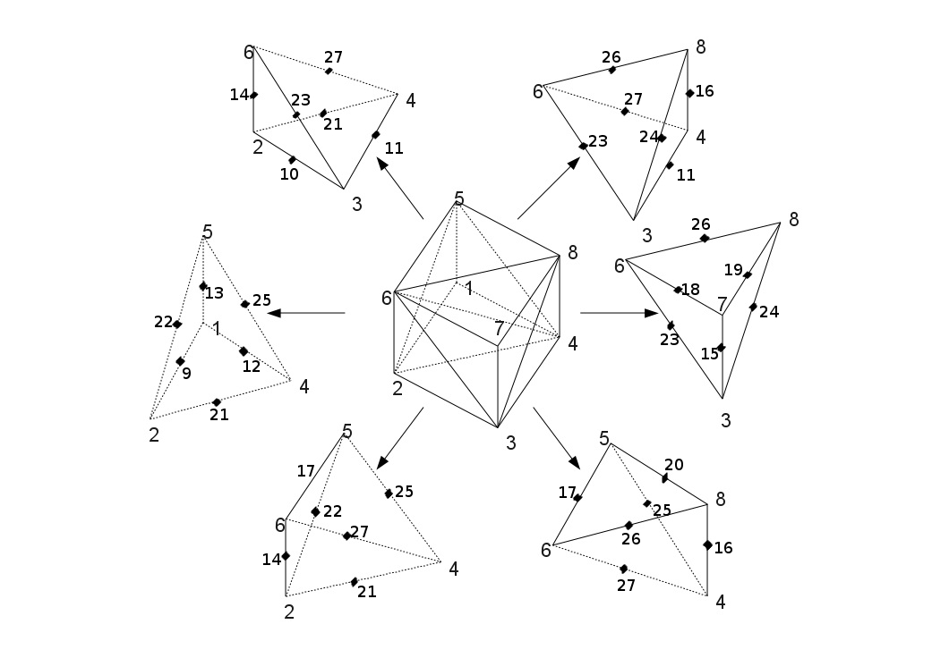
Figure 3.3.1-2 : Division of a quadratic hexahedron (hexa 20) via the complete element (hexa 27)

3.3.2. Preliminary phase of cutting pentahedra to reduce to tetrahedra

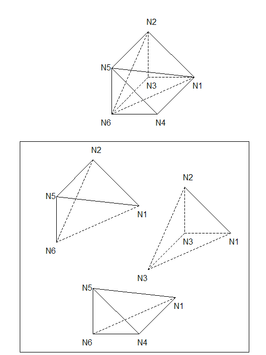
Figure 3.3.2-1 : Diagram for dividing a pentahedron into tetraheders

A pentahedron is then divided into 3 tetrahedra, listed in the following table:

pentahedron	tetrahedron
\(N1N2N3N4N5N6\)	\(N5N4N6N1\)
	\(N1N2N3N6\)
	\(N6N2N5N1\)

Table 3.3.2-1 : Division of a pentahedron into tetraheders

For a quadratic pentahedron (penta15) the above subdivision is retained.

In addition, the middle nodes on the new edges generated by the cut must be taken into account: these middle nodes coincide with the middle nodes of the complete element. We therefore add to the element, the middle nodes necessary to find the complete element.

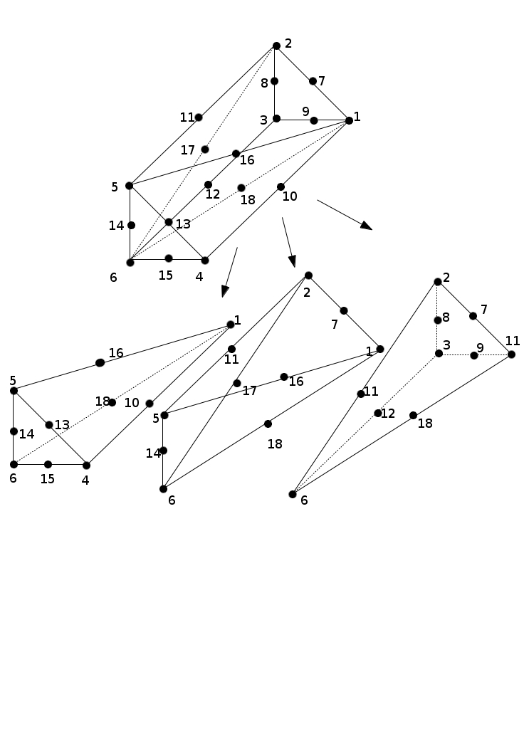
Figure 3.3.2-2: Division of a quadratic pentahedron

3.3.3. Preliminary phase of cutting the pyramids to be reduced to tetrahedra

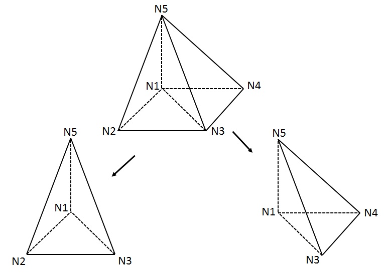
Figure 3.3.3-1 : Diagram of dividing a pyramid into tetraheders

A pyramid is then divided into 2 tetrahedra, listed in the following table:

pyramid	tetrahedron
\(N1N2N3N4N5\)	\(N1N3N4N5\)
	\(N1N2N3N5\)

Table 3.3.3-1 : Dividing a pyramid into tetraheders

For a quadratic pyramid (pyra13) the above subdivision is retained.

In addition, the middle nodes on the new edges generated by the cut must be taken into account: these middle nodes coincide with the middle nodes of the complete element. We therefore add to the element, the middle nodes necessary to find the complete element.

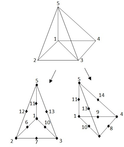
Figure 3.3.3-2: Division of a quadratic pyramid

Note:

L the subdivision of a quadrangle e into two triangles is similar to the subdivision of a pyramid into two tetrahedra.

3.3.4. Sub-division of a tetrahedron into sub-tetrahedra

The reference tetrahedron is set to Figure 3.3.4-1. The intersection points \(\mathit{Pi}\) between the surface \({\mathrm{lsn}}^{h}=0\) and the edges of the tetrahedron are determined.

Let \(n\) be the number of intersection points \(\mathit{Pi}\).

At each intersection point \(\mathit{Pi}\), we associate two integers: \(\mathit{Ai}\) and \(\mathit{NSi}\)

• \(\mathit{Ai}\) is the number of the edge where \(\mathit{Pi}\) is located (for example if \(\mathit{Pi}\) is on the end edge \(\mathit{N2}\mathrm{-}\mathit{N3}\), then \(\mathit{Ai}\mathrm{=}4\)). In the case where \(\mathit{Pi}\) coincides with a vertex node of the tetrahedron, Ai is equal to 0,

• \(\mathit{NSi}\) is the number of the vertex node in the case where \(\mathit{Pi}\) coincides with a vertex node of the tetrahedron (for example if \(\mathit{Pi}\) coincides with \(\mathit{N3}\), then \(\mathit{NSi}\mathrm{=}3\)). In the case where \(\mathit{Pi}\) is on an edge, \(\mathit{NS}\) is equal to 0.

Note:

The product of \(\mathit{Ai}\) by \(\mathit{NSi}\) is always 0.

The intersection points are then sorted in ascending order of \(\mathit{Ai}\). The intersection points coinciding with vertex nodes will therefore be found at the beginning of the list.

Figure 3.3.4-1 : Reference tetrahedron

Since the approximation of the level set uses the shape functions of the tetrahedron, the surface \({\mathit{lsn}}^{h}=0\) is then a plane with linear elements, and a surface with possibly curved geometry, with quadratic elements.

The problem therefore comes down to the cutting of a tetrahedron by a surface. Let’s look at the different possible cases depending on the value of \(n\) (number of intersection points \(\mathit{Pi}\)). We can already eliminate the trivial cases where no sub-division is necessary:

• when \(n<3\) the surface trace in the tetrahedron is a vertex or an edge. If surface \({\mathit{lsn}}^{h}=0\) is not a plane, the geometry of the level-set is then approximated by the edge of the tetrahedron.

• when \(n\mathrm{=}3\) and the 3 points of intersection are vertex points, the trace of the surface in the tetrahedron is one side of the tetrahedron. If surface \({\mathrm{lsn}}^{h}=0\) is not a plane, the geometry of the level-set is then approximated by the face of the tetrahedron.

In these two cases, a single subtetra is obtained, which corresponds to the tetrahedron.

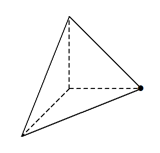
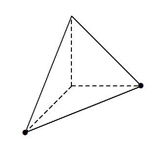
Figure 3.3.4-2 : Case without undercut

\(\mathit{P1}\) and \(\mathit{P2}\) are necessarily the two summit points (so \(\mathit{A1}\mathrm{=}\mathit{A2}\mathrm{=}0\)). Based on \(\mathit{A3}\), the edge number corresponding to \(\mathit{P3}\), we can determine the 2 ends of this edge, that is, \(\mathit{E1}\) and \(\mathit{E2}\).

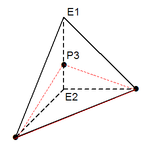
Figure 3.3.4.1-1 : General case where \(n\mathrm{=}3\) including 2 vertex points

One subtetrahedron is obtained on each side of the interface, i.e. in the end 2 subtetrahedra.

2 subtetrahedra

\(\mathit{P1}\mathit{P2}\mathit{P3}\mathit{E1}\) + \(\mathit{P1}\mathit{P2}\mathit{P3}\mathit{E2}\)

Table 3.3.4.1-1 : Sub-tetraheders

To reduce the cutting possibilities, (since there are at least 6 cutting possibilities taking into account the 6 edges in the subtetrahedron) a bijection towards a unique cutting element is constructed. The nodes \(A\), \(B\), \(C\),,, \(D\),,,,,,, \(E\),,, \(F\), \(G\), \(H\) define the unknowns of sequencing of the subtetrahedron cut. Scheduling unknowns will be uniquely associated with the nodes of the parent element. This association constructs a (implicit) bijection.

Recall that,

• scheduling is important from a computer point of view, to ensure the storage of the virtual under-cut mesh. In particular, to locate intersection points and midpoints in data structures XFEM,

• the nodes with a number between 1000 and 1999 represent the intersection points, these nodes are calculated with the procedure described in §4.2.3 of [D4.10.02].

• the nodes with a number greater than 2000 represent the new middle nodes resulting from the cut, these nodes are calculated with the procedure described in §4.2.3 of [D4.10.02]

Note:

For this particular cutting configuration, the construction of the bijection is not**entirely deterministic. In fact, the 2 sub-tetrahedra are symmetric with respect to the cutting plane. From a topological point of view, the unknowns {\(A`*, * ** * ** * ** * **, *:math:`D`*, * *,* *,* :math:`E\) }} are symmetric to the unknowns { \(B\) , \(F\) * , ,, * , , \(G\) }. To make the cutting of a given mesh deterministic, we chose the following arbitrary convention: taking \(A\) as the first node on the edge of the first intersection point.

By analogy to molecular configurations, cutting will potentially generate two configurations called « enantiomers » .

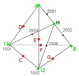
Figure 3.3.4.1-2: cutting element for the configuration 4 intersection points including 2 vertex nodes

\(P1\) is necessarily the summit point (so \(A1=0\) and \(A2\ne 0\)). Edges \(A2\) and \(A3\) have one node in common, \(E1\), and 2 different nodes \(E2\) and \(E3\).

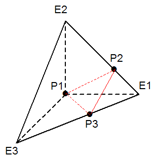
Figure 3.3.4.2-1 : General case where \(n=3\) including a summit point

We obtain a subtetrahedron on one side, and on the other a pyramid that is divided into 2 subtetrahedra, or in the end 3 subtetrahedra.

3 subtetrahedra

\(\mathit{P1}\mathit{P2}\mathit{P3}\mathit{E1}\) + \(\mathit{P1}\mathit{P2}\mathit{P3}\mathit{E3}\) + \(\mathit{P1}\mathit{P2}\mathit{E2}\mathit{E3}\)

Table 3.3.4.2-1 : Sub-tetraheders

To reduce the possibilities of cutting, a bijection is constructed to a unique cutting element. Nodes \(A\), \(B\), \(C\), \(E\),, \(F\),,, \(G\), \(H\) define the sequencing unknowns of subtetrahedron cutting. Scheduling unknowns will be uniquely associated with the nodes of the parent element. This association constructs a (implicit) bijection.

Figure 3.3.4.2-2: cutting element for the configuration 3 intersection points including 1 vertex node

This cutting case corresponds to a flat configuration. This is a particular case of the previous cut for which surface \(\mathit{lsn}=0\) also passes through another vertex node. The cut is then strictly identical to the previous cut (Paragraph [§ 3.3.4.2]). This cutting configuration is represented with on the right the configuration with 3 intersection points and a vertex point to which we refer to*.*

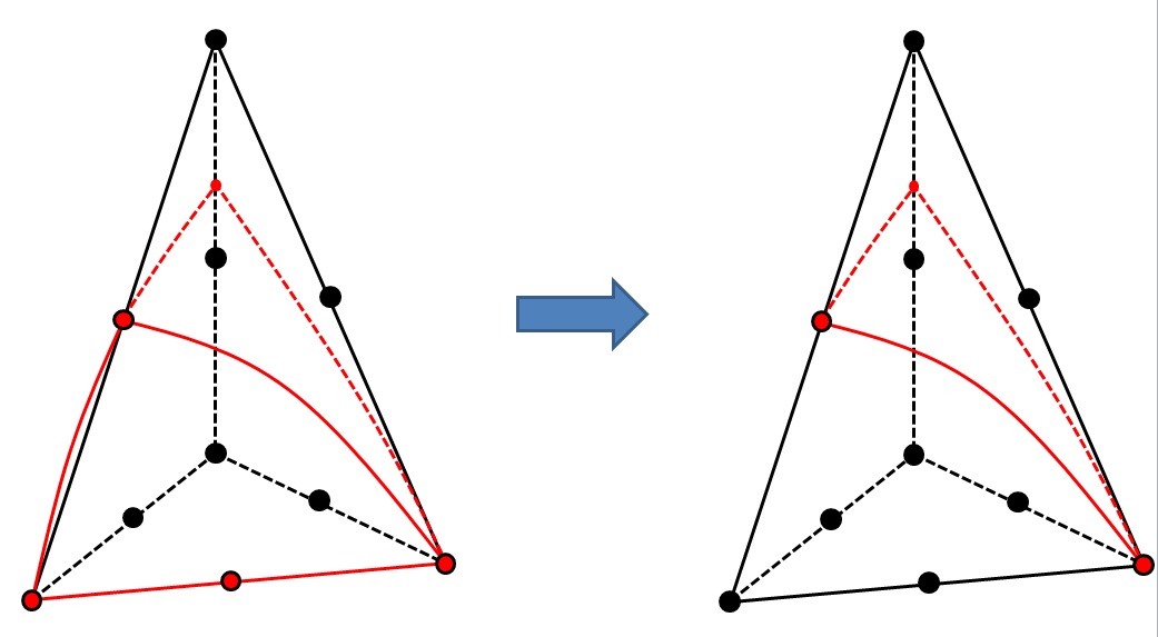
Figure 3.3.4.3-1: Grazing configuration with 5 intersection points (left) and corresponding healthy configuration (right)

There are at least 4 cutting options, listed Figure 3.3.4.4-1. These various possibilities are not treated on a case-by-case basis.

A bijection is constructed to a unique cutting element. Nodes \(A\), \(B\), \(C\), \(D\),, \(E\),,, \(F\), \(G\) define the sequencing unknowns of subtetrahedron cutting. Scheduling unknowns will be uniquely associated with the nodes of the parent element. This association constructs a (implicit) bijection.

Example of identification procedure:

In each of the configurations listed Figure 3.3.4.4-1 , we associate the scheduling unknowns n œ*uds* \(\text{{}A,B,C,D\text{}}\) with the n œ*uds* \(\text{{}{N}_{\mathrm{1,}}{N}_{\mathrm{2,}}{N}_{\mathrm{3,}}{N}_{4}\text{}}\) of the sub-tetrahedron. As the node \(A\) belongs to the three cut edges, it is easily identified with the corresponding node in each of the configurations listed. Then, we then identify \(\text{{}B,C,D\text{}}\) since the n œ*uds* \(B\) , \(C\) , \(D\) belong respectively to the first, second, third intersected edge, and are different from the node \(A\) previously identified. The result is the correspondence table

This identification procedure makes it possible to construct a bijection implicitly.

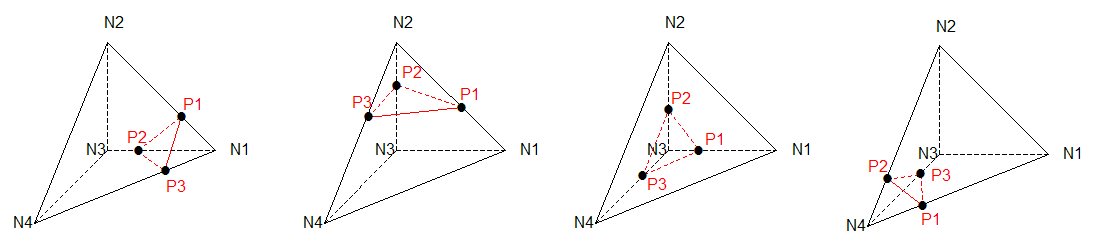
Figure 3.3.4.4-1: Configurations of a tetrahedron with 3 intersecting edges

Figure 3.3.4.4-2: cutting element for the configuration with 3 intersection points and no vertex nodes

From to
\((A,B,C,D)\)	\(({N}_{\mathrm{1,}}{N}_{\mathrm{2,}}{N}_{\mathrm{3,}}{N}_{4})\)
\((A,B,C,D)\)	\(({N}_{\mathrm{2,}}{N}_{\mathrm{1,}}{N}_{\mathrm{3,}}{N}_{4})\)
\((A,B,C,D)\)	\(({N}_{\mathrm{3,}}{N}_{\mathrm{1,}}{N}_{\mathrm{2,}}{N}_{4})\)
\((A,B,C,D)\)	\(({N}_{\mathrm{4,}}{N}_{\mathrm{1,}}{N}_{\mathrm{2,}}{N}_{3})\)

Table 3.3.4.4-1: Identifying the nodes of the cutting element to the nodes of the subtetrahedron in each configuration

This cutting case corresponds to a flat configuration. This is a particular case of the previous cut for which surface \(\mathit{lsn}=0\) also passes through one of the vertex nodes. The cut is then strictly identical to the previous cut (Paragraph [§ 3.3.4.4] ). This cutting configuration is represented with, on the right, the configuration with 3 intersection points to which we refer.

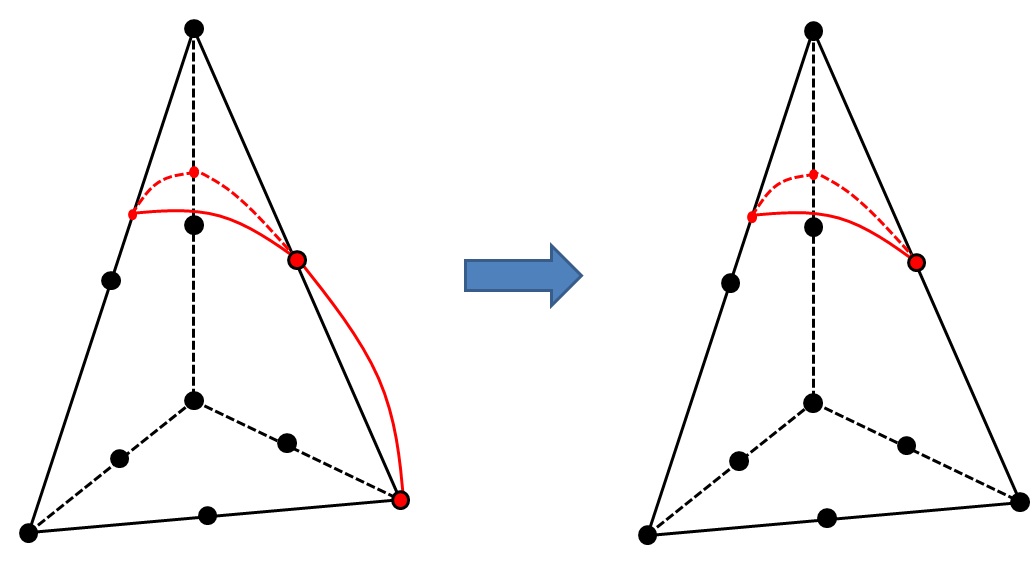
Figure 3.3.4.5-1: Grazing configuration with 4 intersection points (left) and corresponding healthy configuration (right)

This cutting case corresponds to a flat configuration. This is another particular case of the previous cut for which surface \(\mathit{lsn}=0\) also passes through two of the vertex nodes. The cut is then strictly identical to the previous cut (Paragraph [§ 3.3.4.4]). This cutting configuration is represented with, on the right, the configuration with 3 points of intersection to which we refer to*.*

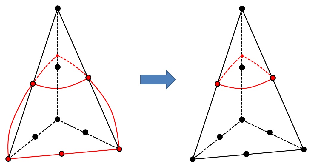
Figure 3.3.4.6-1: Grazing configuration with 6 intersection points (left) and corresponding healthy configuration (right)

There are at least 3 cutting options, listed. These various possibilities are not treated on a case-by-case basis.

A bijection is constructed to a unique cutting element. Nodes \(A\), \(B\), \(C\), \(D\),, \(E\), \(F\), define the sequencing unknowns of subtetrahedron cutting. Scheduling unknowns will be uniquely associated with the nodes of the parent element. This association constructs a (implicit) bijection.

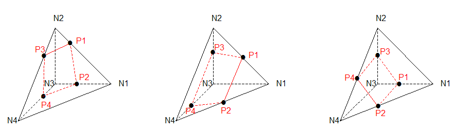
Figure 3.3.4.7-1: Configurations of a tetrahedron with 4 intersecting edges

Figure 3.3.4.7-2: cutting element for the configuration with 4 intersection points and no vertex nodes

This cutting case corresponds to a flat configuration. This is a particular case of the previous cut for which surface \(\mathit{lsn}=0\) also passes through one of the vertex nodes. The cut is then strictly identical to the previous cut (Paragraph [§ 3.3.4.7]). This cutting configuration is represented with, on the right, the configuration with 4 intersection points to which we refer.

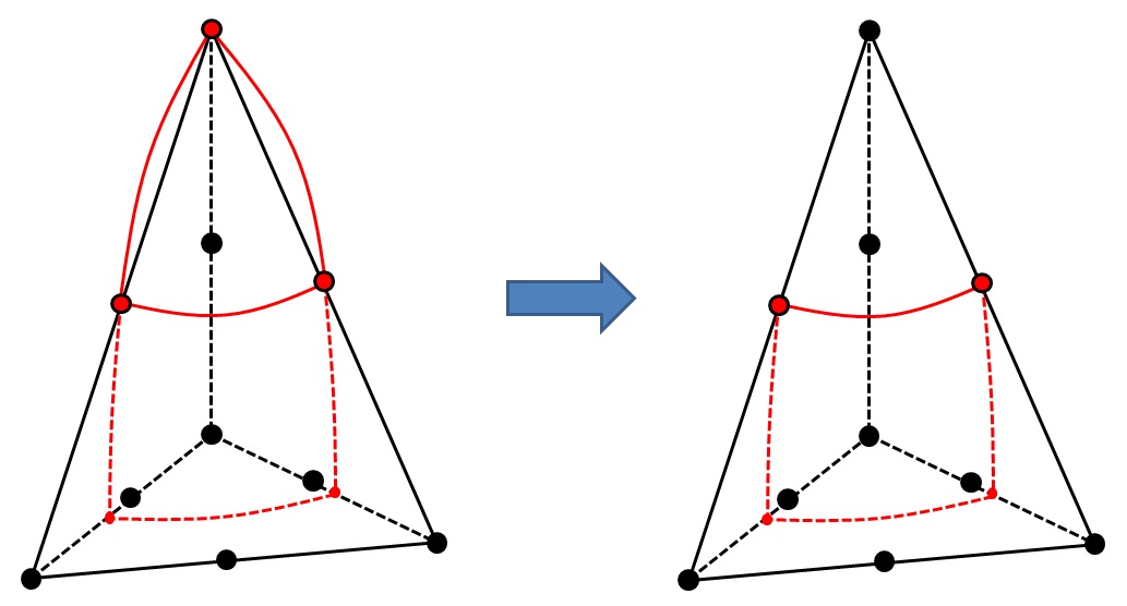
Figure 3.3.4.8-1: Grazing configuration with 5 intersection points (left) and corresponding healthy configuration (right)

This cutting configuration corresponds to a flat configuration. It does not boil down to any configuration previously described. It can be distinguished from the configuration described in Paragraph [§ 3.3.4.5]) (which also includes 4 intersection points including a vertex point) because the vertex node not intersected on the grazing edge belongs to only two intersected edges (instead of 3 in the case described in Paragraph [§ 3.3.4.5]). There are at least 24 cutting options, 3 of which are listed in the. These various possibilities are not treated on a case-by-case basis.

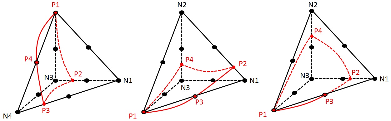
Figure 3.3.4.9-1: Configurations of a tetrahedron with 4 intersection points including a vertex point

A bijection is constructed to a unique cutting element. Nodes \(A\), \(B\), \(C\), \(D\),, \(E\), \(F\), define the sequencing unknowns of subtetrahedron cutting. Scheduling unknowns will be uniquely associated with the nodes of the parent element. This association constructs a (implicit) bijection. This cutting configuration gives rise to 5 child subtetrahedra.

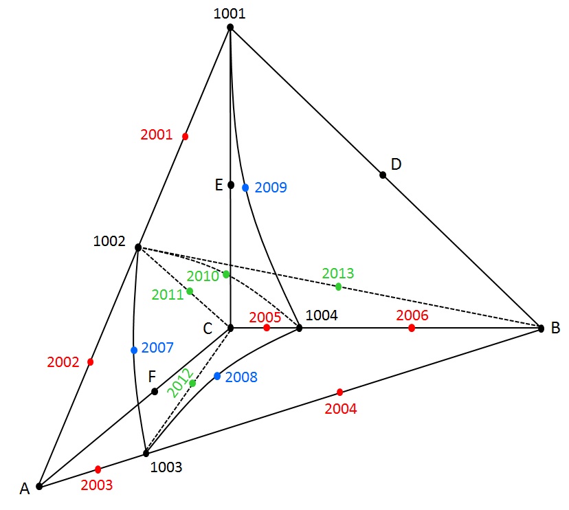
Figure 3.3.4.9-2: cutting element for the configuration with 4 intersection points including a vertex node

3.3.5. Multi-die-cutting

When you want to model junctions, intersections or simply that two cracks are close enough to cut the same element, you must be able to divide the element into domains that respect all the discontinuities introduced.

The strategy adopted consists in cutting the element several times sequentially. This is a strategy that has the merit of being fairly quick to implement, because the cutting of a reference tetrahedron by a crack generates sub-tetrahedra which can in turn be considered as reference tetrahedra for cutting by the next crack.

The problem is that we do not optimize the total number of sub-elements generated, which may be very high if we recut more than 3 times in 3D. To solve this problem, it would be necessary to be able to directly cut any type of element (hexahedron, pentahedron, pyramid, tetrahedron) in combination of all these types of elements. This requires fairly heavy developments and is therefore not an option. Another strategy would be to group sub-items by zone and find the optimal number of Gauss points (and weights) per zone. We would no longer store the sub-elements but directly the areas with the associated gauss points.

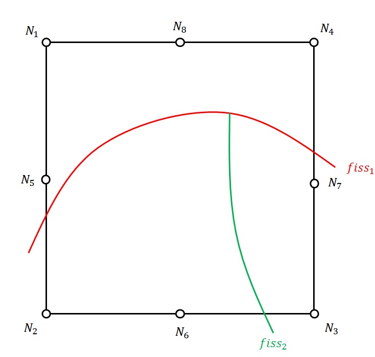
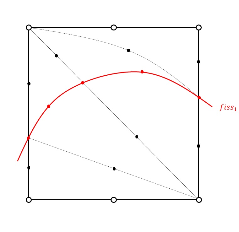
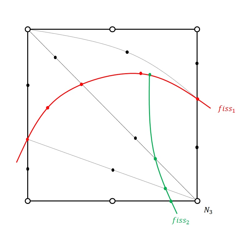
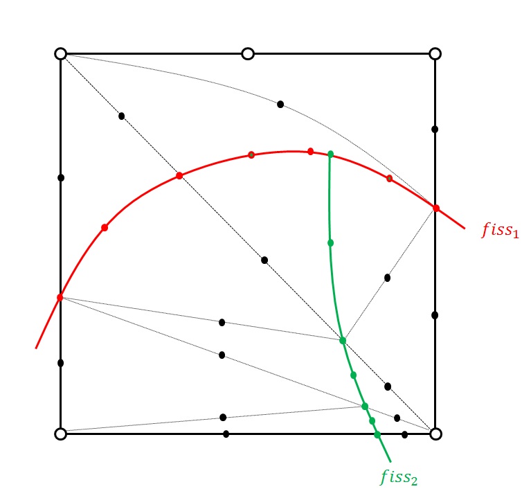
Figure 3.3.5-1: Example of multi-division in 2D

3.3.6. Maximum number of sub-items

In order to correctly size the data structures relating to the sub-division, it is necessary to determine the maximum number of sub-elements generated by the sub-division phase, according to the type of the initial mesh.

In this paragraph, it is considered that the element is cut by only one crack.

The case with the largest number of sub-elements is the one described in paragraph [§ 3.3.4.7], which results in 6 sub-elements.

A pentahedron being previously divided into three tetrahedra, one might think that the largest number of sub-elements generated is where each of these three tetrahedra is in turn sub-divided into 6 sub-elements; which would result in a final division into 18 sub-elements. This would lead to a final division into 18 sub-elements. However, such a scenario is impossible. At most, out of the three tetrahedra, two will be divided into 6 sub-elements and only one will be divided into 4 sub-elements, resulting in 16 sub-elements.

As before, the case where all the six tetrahedra are each sub-divided into 6 sub-elements is impossible. The maximum case is the one that corresponds to the case mentioned in the previous paragraph: the two pentahedra deduced from the hexahedron (see Figure 3.3.1-1) are each sub-divided into 16 sub-elements. So the number of sub-elements is \((6+6+4)+(6+6+4)=32\).

A finite element XFEM can be cut by a maximum of 4 cracks in codeaster. The maximum number of sub-elements generated is then difficult to evaluate and an increase in the maximum number of sub-elements would be too high. In fact, if we take the maximum number of sub-elements generated by a single crack, i.e. 32, and if we consider that the 32 tetrahedra can give rise to 6 tetrahedra for each of the following cracks, we obtain \(32\ast \mathrm{6³}=6912\). This number of integration sub-elements for a hexahedron is completely unattainable because it goes without saying that the tetrahedra resulting from the first division will not all be cut by the following cracks, but it is difficult to show a better major component. The choice is made to set the maximum number of sub-elements for multi-cracked elements to 4 times the maximum number of sub-elements for a single crack, i.e. \(32\ast 4=128\) in 3D and \(4\ast 6=24\) in 2D. These numbers can easily be exceeded for elements cut by 3 or 4 cracks. In this case, the cutting procedure returns an error and the user is invited to refine the mesh used in order to avoid that finite elements are streaked with cracks, which would also lead to major packaging problems (see paragraph [§ 3.2.6]).

3.3.7. 2D subdivision

A method comparable to 3D cutting is used for 2D cutting. The quadrangles will be subdivided into triangles that are themselves subdivided according to the passage of the crack.

We cut the quadrangles into 2 triangles:

Figure 3.3.7-1 : Subdivision of a quadrangle into triangles: linear (left), quadratic (right)

quadrangles	triangles
\(\mathit{N1}\mathit{N2}\mathit{N3}\mathit{N4}\)	\(\mathit{N1}\mathit{N2}\mathit{N4}\)
	\(\mathit{N2}\mathit{N3}\mathit{N4}\)
\(\mathit{N1}\mathit{N2}\mathit{N3}\mathit{N4}\mathit{N5}\mathit{N6}\mathit{N7}\mathit{N8}\)	\(\mathit{N1}\mathit{N2}\mathit{N4}\mathit{N5}\mathit{N9}\mathit{N8}\)
	\(\mathit{N2}\mathit{N3}\mathit{N4}\mathit{N6}\mathit{N7}\mathit{N9}\)

Then the triangles are intersected according to the passage of the crack. We perform the same sorting as in 3D for the intersection points \(\mathit{Pi}\).

Note:

Node \(N9\) is not a mesh node. It is added to make the connectivity between the quadrangle and the quadratic triangles. It is defined as the middle of the segment \(N2N4\) (and not the center node of the quadrangle). The value of the normal level set assigned to it is obtained by interpolating the \(\mathit{lsn}\) nodes \(N1\) to \(N8\). A readjustment may then be necessary to ensure the uniqueness of the solution of the equation \(\mathit{lsn}=0\) along the diagonal (cf. readjusting the level sets [§ 2.2.4 ]) when dividing the child elements into integration sub-elements. Prior to any cutting, we therefore loop the edges of the child elements (this has already been done for the edges of the parent elements when readjusting the level sets) to detect pathogenic situations and make the necessary readjustments, exactly as described in [§ 2.2.4 ] .

When you have 1 or 2 intersection points that fall only on the vertices, no division is necessary.

Figure 3.3.7-2 : Case without undercut

If 1 or 2 of the intersection points do not fall on a vertex, the triangles are intersected.

If you have 1 vertex point and 1 non-vertex point, \(\mathit{P1}\) is necessarily vertex. We determine the vertices of the edge of the 2nd point \(\mathit{N2}\) and \(\mathit{N3}\) to cut the triangle into 2 sub-triangles \(\mathit{P1}\mathit{N2}\mathit{P2}\) and \(\mathit{P1}\mathit{N3}\mathit{P2}\). If the triangle is quadratic, we determine the midpoints of the edge of the 2nd point \(\mathit{Q1}\) and \(\mathit{Q2}\) and that of the crack \(\mathit{Q3}\).

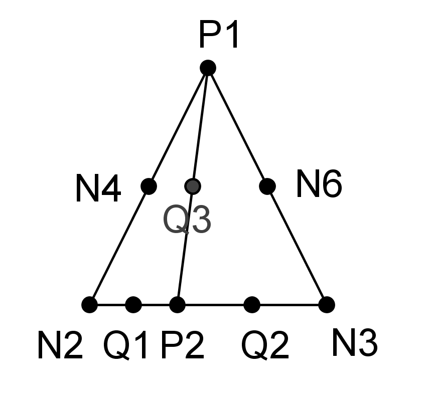
Figure 3.3.7-3 : Case of linear (left) and quadratic (right) division **** with 2 intersection points including 1 vertex **

With 2 non-vertex points, you have to cut into 3 triangles. We get triangles \(\mathit{N1}\mathit{P1}\mathit{P2}\), \(\mathit{P1}\mathit{P2}\mathit{N3}\), and \(\mathit{P1}\mathit{N2}\mathit{N3}\). \(\mathit{N1}\) being the point close to the 2 intersection points according to the sorting done. If the triangle is quadratic, we determine the midpoints of the edge of the 1st point \(\mathit{Q1}\) and \(\mathit{Q2}\), those of the 2nd point \(\mathit{Q3}\) and \(\mathit{Q4}\), that of the crack \(\mathit{Q5}\) and that of the new edge \(\mathit{Q6}\).

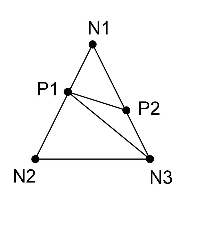
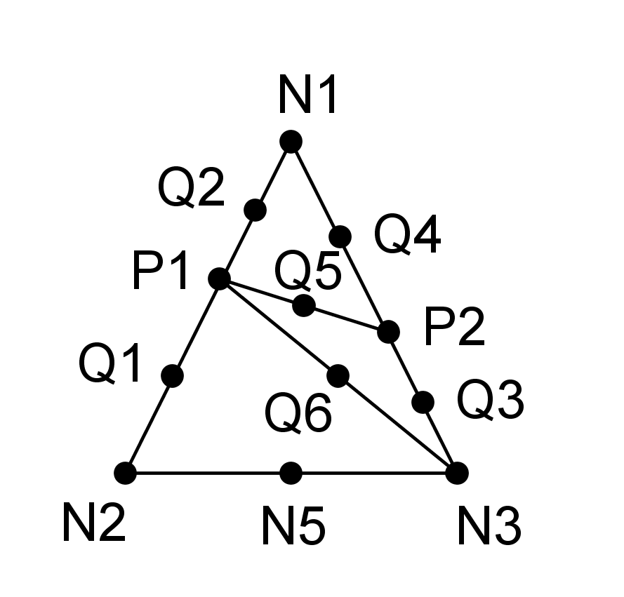
Figure 3.3.7-4 : Case of linear (left) and quadratic (right) division with 2 intersection points without vertex

3.3.8. Sub-slicing algorithms

In paragraphs § 3.3.1 to § 3.3.7, we explained the geometric division of elements into integration sub-cells (Tetra10 in 3D, Tri6 in 2D), without explaining how the coordinates of the intersection points and of the new middle nodes in the virtual mesh are calculated. In this paragraph, we will therefore describe the algorithms for calculating the coordinates of the new points, generated by the cut.

For each type of point, there is a specific positioning algorithm:

• The positioning of the intersection points allows an explicit border to be delineated, although the interface/crack is defined by an implicit equation \({\mathrm{lsn}}^{h}=0\). Precisely, the location of the intersection points is calculated by taking the intersection between the edges of the mesh and the iso-zero of the level-set. The intersection points are then stored in an auxiliary data structure, in addition to the points of the [D4.10.02] mesh.

• The positioning of the midpoints makes it possible to improve the description of a level-set curve, in the case of quadratic elements. In the presence of elements with curved edges, the curvature of the edges of the quadratic element is maintained, by positioning middle nodes rigorously on the edges during cutting. On the other hand, a cut with elements with straight edges would alter the curvature of the original element. To capture the curvature of the level-set and the curved edges of quadratic elements, we therefore calculate several types of midpoints (see § Error: Reference source not found). Several algorithms are implemented to capture the different types of possible midpoints. These new midpoints are then stored in an auxiliary data structure, in addition to the points of the mesh [D4.10.02].

Thereafter, the following notation is adopted:

• \(\xi ={\left({\xi }_{i}\right)}_{i\in [\mathrm{1,}\mathit{dim}]}\) refers to the reference coordinates in the parent element. These coordinates generally vary between \(\left[\mathrm{0,1}\right]\) and \(\left[-1,1\right]\). Recall that shape functions or interpolation polynomials are parameterized in Aster, using the reference coordinates [R3.01.01],

• \(X={\left({X}_{i}\right)}_{i\in [\mathrm{1,}\mathit{dim}]}\) refers to the coordinates of a point in real space. If the current point is a node, these are the geometric coordinates of the node in the mesh. If the current point is not a node, it is the geometric coordinates interpolated into the parent element \(X(\mathrm{\xi })=\sum _{1⩽j⩽\mathit{nnop}}{X}^{j}{\mathrm{\Phi }}_{j}(\mathrm{\xi })\).

14. Moës proposes to pose the problem of finding intersection points in the parent reference space. Clearly, to calculate the real coordinates of a point of intersection, we first search for the coordinates in the reference space \(\xi\). The real coordinates are then deduced by interpolating the geometric coordinates in the parent element.

To calculate the intersection point \(P\) between an edge \(\mathit{AB}\) and the iso-zero, we solve the following problem:

\(\begin{array}{c}P\in \mathit{AB}\\ {\mathit{lsn}}^{h}\left(P\right)=0\end{array}\)

Figure 3.3.8.1-1: Find the intersection point \({I}_{1}\) on edge \({I}_{2}{I}_{3}\) which is curved in the reference space. We then take in

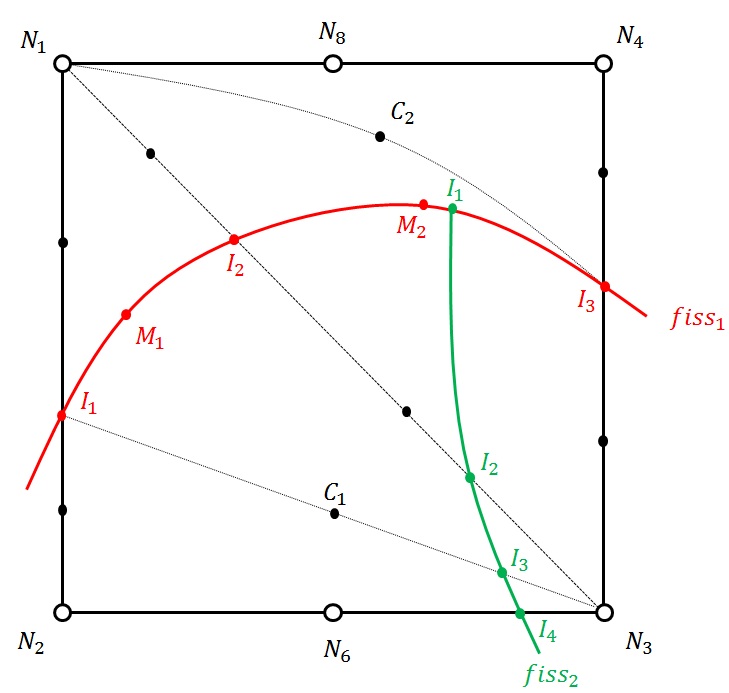
Count the curvature of \({I}_{2}{I}_{3}\) with the middle node \({M}_{2}\)

Exception: For multi-cracked quadratic elements, in the parent reference element, edge \(\mathit{AB}\) is not necessarily straight. The middle node \(M\) of the edge \(\mathit{AB}\) is not necessarily on the segment \([A,B]\) if the side \(\mathit{AB}\) is the side of an integration sub-element generated by the cut in accordance with a first crack (see). It is then necessary to take into account the possible curvature of the edge; we thus have \(P\in \mathit{AB}\iff {\xi }_{P}=(\mathrm{2t}-1)(t-1){\xi }_{A}+t(\mathrm{2t}-1){\xi }_{B}+\mathrm{4t}(1-t){\xi }_{M}\) with \(t\in [:ref:`0,1 <0,1>\)] `.

So, the problem posed is to search for \(t\in [\mathrm{0,}1]\) such as \({\mathit{lsn}}^{h}\left({\xi }_{P}=(\mathrm{2t}-1)(t-1){\xi }_{A}+t(\mathrm{2t}-1){\xi }_{B}+\mathrm{4t}(1-t){\xi }_{M}\right)=0\).

For mono-fissured linear or quadratic models, point \(P\) necessarily belongs to edge \([A,B]\) and therefore: \({\xi }_{P}=(1-t){\xi }_{A}+t{\xi }_{B}\) with \(t\in [:ref:`0,1 <0,1>\)] `.

So, the problem posed is to search for \(t\in [\mathrm{0,}1]\) such as \({\mathit{lsn}}^{h}\left({\xi }_{P}=(1-t){\xi }_{A}+t{\xi }_{B}\right)=0\).

We then look for the root of a polynomial equation since the interpolation functions of the level-set are polynomials. This equation is then solved using the Newton-Raphson algorithm (detailed below).

As \(f\mathrm{:}t\to {\mathit{lsn}}^{h}(t)\) is \({C}^{2}\) and strictly monotonic in the vicinity of the intersection point (otherwise, the level-set becomes parallel to edge \(\mathit{AB}\) and does not intersect it), the convergence of Newton’s algorithm is quadratic, and therefore optimal.

Newton-Raphson algorithm for calculating a point where iso-zero intersects with the edge \(\mathit{AB}\) :

• Reading the reference coordinates of the \(A\) and \(B\) vertex nodes and of the possible middle node \(M\): by construction, these nodes are nodes of the child element that is being cut and their coordinates are therefore known.

• Newton-Raphson initialization:

\({t}_{0}=\frac{\mathit{lsn}(A)}{\mathit{lsn}(A)-\mathit{lsn}(B)}\)

---

\(\mathit{lsn}(A)+(4\ast \mathit{lsn}(M)-3\ast \mathit{lsn}(A)-\mathit{lsn}(B))\ast {t}_{0}+2\ast (\mathit{lsn}(A)+\mathit{lsn}(B)-2\ast \mathit{lsn}(M))\ast {t}_{0}\mathrm{²}=0\)

Among the two possible solutions to this quadratic equation, only the one that satisfies is retained: \({t}_{0}\in [:ref:`0,1 <0,1>\)] . This value is a good initialization and is even the final solution to the problem when the edge of the child element on which the search is performed coincides with an edge of the parent element. In fact, l :math:mathit{lsn}` is then interpolated only by the end and middle nodes of the edge of the parent element. Since this interpolation is quadratic, initialization provides the exact solution. In contrast, when the edge of the child element does not coincide with an edge of the parent element (inner edge), initialization does not provide the exact solution to the problem because \(\mathit{lsn}\) is interpolated by all the nodes of the parent element along the edge of the child element.

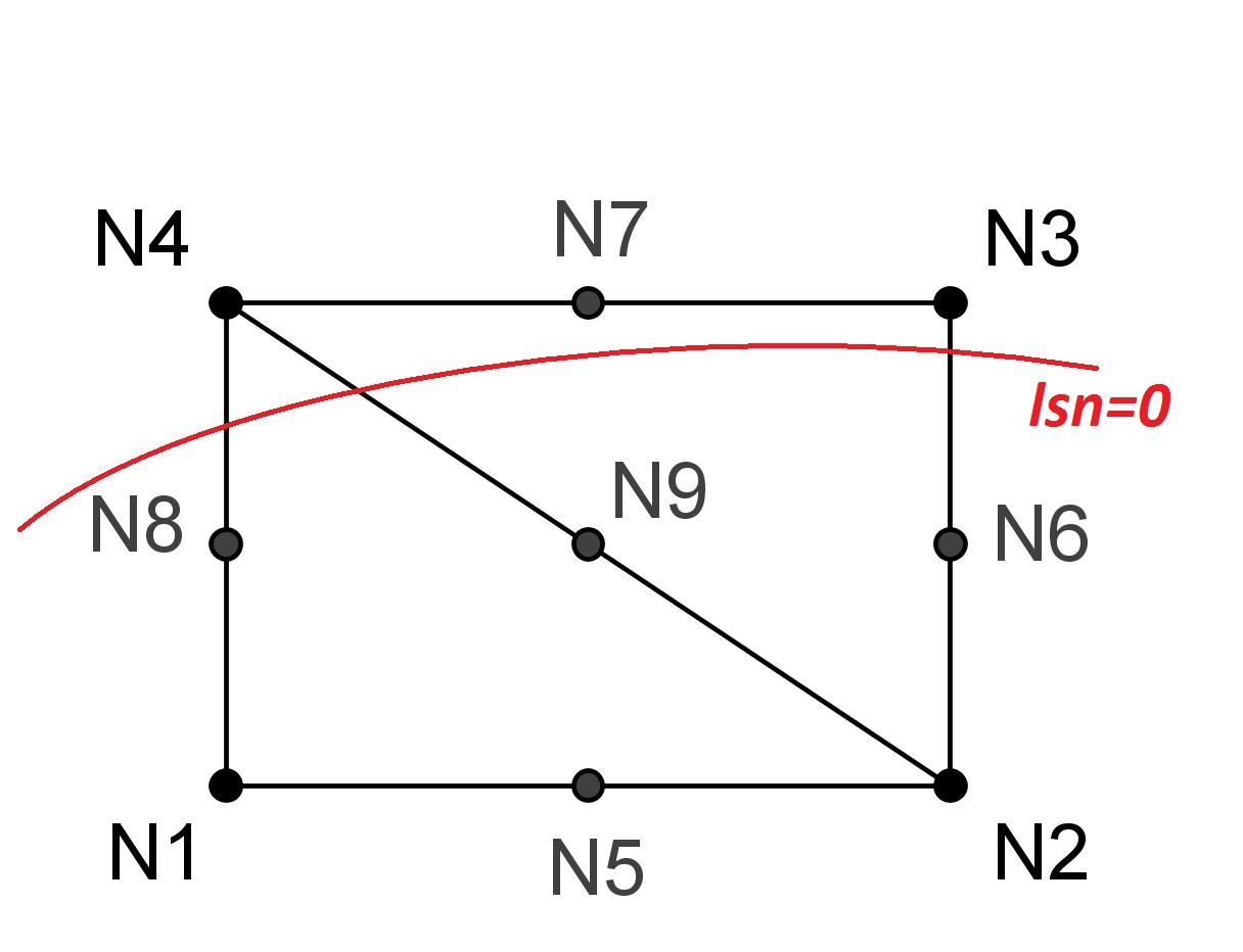
Figure 3.3.8.1-2: Intersection of the*lsn=0* curve with an edge of the child element

• As long as \(n⩽\mathit{itermax}\) do:

  • \({\xi }_{n}=\{\begin{array}{c}(1-{t}_{n}){\xi }_{A}+{t}_{n}{\xi }_{B}\text{}\mathit{en}\mathit{linéaire}\mathit{et}\mathit{mono}-\mathit{fissuré}\\ ({\mathrm{2t}}_{n}-1)({t}_{n}-1){\xi }_{A}+{t}_{n}({\mathrm{2t}}_{n}-1){\xi }_{B}+{\mathrm{4t}}_{n}(1-{t}_{n}){\xi }_{M}\text{}\mathit{en}\mathit{quadratique}\mathit{multi}-\mathit{fissuré}\end{array}\)

  • Calculating the function: \({\mathit{lsn}}^{h}({\xi }_{n})=\sum _{1⩽j⩽\mathit{nnop}}{\mathit{lsn}}_{j}{\Phi }_{j}({\xi }_{n})\)

  • Calculation of the derivative: \({\mathit{dlsn}}^{h}({\xi }_{n})/\mathit{dt}=\sum _{1⩽j⩽\mathit{nnop}}{\mathit{lsn}}_{j}\nabla {\Phi }_{j}({\xi }_{n})\cdot \vec{v}\)

  • Slope check: if \(∣{\mathit{dlsn}}^{h}({\xi }_{n})/\mathit{dt}∣<{10}^{-16}\) then exit with error code.

  • Calculating the increment: \({\Delta }_{n}=\frac{{\mathit{lsn}}^{h}({\xi }_{n})}{{\mathit{dlsn}}^{h}({\xi }_{n})/\mathit{dt}}\)

• Verification of hypothesis \(\mathit{AB}\): if \({t}_{n}\notin \left[\mathrm{0,1}\right]\) then exit with error code.

• Criterion for stopping the increment: if \(∣{\Delta }_{n}∣<{10}^{-8}\) then end of the loop.

• Calculation of the reference coordinates of the intersection point: \({\xi }_{\infty }=\{\begin{array}{c}(1-{t}_{\infty }){\xi }_{A}+{t}_{\infty }{\xi }_{B}\text{}\mathit{en}\mathit{linéaire}\mathit{et}\mathit{mono}-\mathit{fissuré}\\ ({\mathrm{2t}}_{\infty }-1)({t}_{\infty }-1){\xi }_{A}+{t}_{\infty }({\mathrm{2t}}_{\infty }-1){\xi }_{B}+{\mathrm{4t}}_{\infty }(1-{t}_{\infty }){\xi }_{M}\text{}\mathit{en}\mathit{quadratique}\mathit{multi}-\mathit{fissuré}\end{array}\)

• Verification of hypothesis \(P\in \mathit{ELREFP}\): if \({\xi }_{\infty }\notin \mathit{ELREFP}\) then exit with error code.

• Calculation of real coordinates by interpolation of geometric coordinates:

\(X({\xi }_{\infty })=\sum _{1⩽j⩽\mathit{nnop}}{X}^{j}{\Phi }_{j}({\xi }_{\infty })\)

Note on the stopping criterion:

We test the increment \({\Delta }_{n}\) to assess Newton’s convergence, because the solution and the increment vary on the unity scale. The value of the increment in relation to the unit is therefore a robust indicator of convergence. If the stopping criterion was based on the value of the function \({\mathit{lsn}}^{h}({\xi }_{n})\) , the result should be scaled.

Very concretely, when the increment tends to zero with respect to unity, the solution \({t}_{n+1}={t}_{n}-{\Delta }_{n}\) becomes stationary with respect to unity. From a numerical point of view, this guarantees convergence over the range \([0,1]\) , taking into account machine precision.

As an example, let’s now consider the interpolation of a level-set into the quadratic element (QUAD8) in paragraph § 2.2.3. Consider an arbitrary \(\mathit{AB}\) segment in the parent element (see). By plotting the evolution of the interpolated level-set \(f\mathrm{:}t\to {\mathit{lsn}}^{h}(t)\) along the segment \(A\text{-}B\) (see), we see that the level-set varies in a strictly monotonic manner in the vicinity of the intersection point \(P\). As long as we remain in the vicinity of point \(P\), Newton’s algorithm will respect the conditions of optimal convergence.

The Newton algorithm proposed above is initialized by a linear interpolation of the level-set along segment \(A\text{-}B\). The initialization point \({P}_{0}\) is then sufficiently close to the convergence point \(P\). Newton’s algorithm will have optimal behavior.

On the other hand, if the algorithm had been initialized at point \(A\), the proximity of a stationary point (where the first derivative of \(f\mathrm{:}t\to {\mathit{lsn}}^{h}(t)\) cancels out) would have caused Newton to fail. Several scenarios would be possible:

• or the Newton would not converge after a given maximum number of iterations,

• or the Newton would leave segment \(A\text{-}B\).

The presence of the stationary point has a geometric justification: the iso-zero of the level-set is practically parallel to segment \(A\text{-}B\) in the vicinity of point \(A\) (see). Thereafter, the distance between segment \(A\text{-}B\) and the iso-zero decreases progressively. Consequently, in the vicinity of the intersection point, the variation in the level-set becomes strictly monotonic again.

To prevent this configuration, Newton is initialized sufficiently close to the point of intersection. In addition, at each iteration of the algorithm, we check the persistence of the solution on segment \(A\text{-}B\), i.e. \(\forall t,t\in [:ref:`0,1 <0,1>\)] `. This then provides an additional guarantee on the robustness of the solution calculated by Newton.

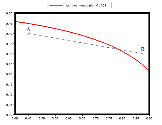
Figure 3.3.8.1-3: Finding the intersection point between the iso-zero of the level-set and an A-B (arbitrary) segment in an element QUAD8

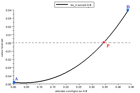
Figure 3.3.8.1-4: evolution of the distance function (level-set) along the A-B segment

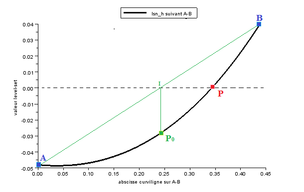
Figure 3.3.8.1-5: Initialization of the Newton-Raphson algorithm by linear interpolation of the level-set

When cutting a quadratic tetrahedron, the new midpoints can be grouped into 3 categories:

• the middle points of the first type \({\mathit{MP}}_{1}\): located on the edges of the tetrahedron (triangle), between the intersection points and the vertex nodes,

• the middle points of the second type \({\mathit{MP}}_{2}\): located on the iso-zero, in the quadratic face (SE3, TRI6 or QUAD8) delimited by the intersection points. The midpoints at the edges of the face and the midpoint at the center of the face (if the face is quadrangle) are calculated using slightly different procedures,

• the middle points of the third type \({\mathit{MP}}_{3}\): located on the quadrangle faces of the child sub-polyhedra (pentahedron or pyramid), generated by the cutting of the tetrahedron.

Figure 3.3.8.2-1: the different types of middle nodes \({\mathit{MP}}_{i}\) to be calculated when cutting quadratic elements

Definition of midpoints

It is proposed to systematically define the midpoints in the reference frame of the parent element. As the reference element has straight edges and flat faces, this greatly facilitates the calculation of midpoints, especially first-type middle nodes. Let us emphasize this essential point further, future calculations will often be based implicitly on the assumption that the faces of the tetrahedra to be cut are flat in the parent reference element.

However, with this definition, it is possible to calculate a middle node that is not « in the middle » of the edge in the real coordinate system. This is not a problem, provided you choose a suitable integration technique.

In the reference element, we propose the following definition of midpoints:

• for a midpoint of the**first type**, located between the vertex node \(\mathit{XX}\) and the intersection point \(\mathit{IP}\): \({\xi }_{{\mathit{PM}}_{1}}={\xi }_{\mathit{Milieu}(\mathit{XX}\text{-}\mathit{IP})}=\frac{{\xi }_{\mathit{XX}}+{\xi }_{\mathit{IP}}}{2}\)

As shown on the.

Figure 3.3.8.2-2: calculation in the reference coordinate system, of a middle point of the second type, located between 2 intersection points

Exception: For multi-cracked quadratic elements, in the parent reference element, the intersected edge on which you want to position the midpoints is not necessarily straight. If the intersected edge is the side of an integration sub-element generated by the cut in accordance with a first crack (see), the possible curvature of the edge must be taken into account in order to position the middle points of the first type:

\(\begin{array}{c}{\xi }_{{M}_{6}}=\frac{{\xi }_{{I}_{4}}+{\xi }_{{I}_{2}}}{2}\\ {M}_{6}=\frac{{\xi }_{{M}_{6}}({\xi }_{{M}_{6}}-1)}{2}{I}_{2}+\frac{{\xi }_{{M}_{6}}({\xi }_{{M}_{6}}+1)}{2}{I}_{3}+(1-{\xi }_{{M}_{6}})(1+{\xi }_{{M}_{6}}){I}_{4}\end{array}\)

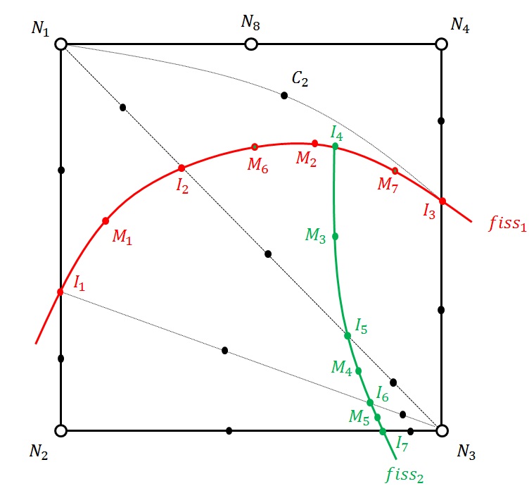
Figure 3.3.8.2-3: determination of midpoints \({M}_{6}\) and \({M}_{7}\) on edge \({I}_{2}{I}_{3}\)

• for a midpoint of the**second type**, located between 2 intersection points on one side of the tetrahedron, the following choice is made:

\(\begin{array}{c}{\xi }_{{\mathit{PM}}_{2}}={\xi }_{M}+t\vec{v}\\ {\mathit{lsn}}^{h}\left({\xi }_{{\mathit{PM}}_{2}}\right)=0\end{array}\)

Figure 3.3.8.2-4: calculation in the reference coordinate system, of a middle point of the second type, located between 2 intersection points

• \(\vec{v}\) is the unit vector normal to \(\vec{{\mathit{IP}}_{1}\text{-}{\mathit{IP}}_{2}}\), belonging to the face \((A,B,C)\) (plane in the reference element). Concretely to calculate the normal vector \(\vec{v}\), we ask the following equations:

\(\left\{\begin{array}{c}\vec{v}\text{}\in \text{}(A,B,C)\\ \vec{v}\text{}\perp \text{}\vec{{\mathit{IP}}_{1}\text{-}{\mathit{IP}}_{2}}\\ \parallel \vec{v}\parallel \text{}=\text{}1\end{array}\right\}\Rightarrow \left\{\begin{array}{c}\vec{v}\text{}=\text{}{\alpha }_{1}\vec{\mathit{AB}}\text{}+\text{}{\alpha }_{2}\vec{\mathit{AC}}\\ \vec{v}\text{}\cdot \text{}\vec{{\mathit{IP}}_{1}\text{-}{\mathit{IP}}_{2}}\text{}=\text{}0\\ \parallel \vec{v}\parallel \text{}=\text{}1\end{array}\right\}\)

After resolution:

\(\vec{v}\text{}=\text{}\pm {\alpha }_{1}\left({k}_{2}\vec{\mathit{AB}}\text{}-\text{}{k}_{1}\vec{\mathit{AC}}\right)\) with \(\begin{array}{c}{\alpha }_{1}\text{}=\text{}1/\sqrt{{n}_{1}^{2}{k}_{2}^{2}+{n}_{2}^{2}{k}_{1}^{2}-2k{k}_{1}{k}_{2}}\\ {n}_{1}\text{}=\text{}\parallel \vec{\mathit{AB}}\parallel \text{et}{n}_{2}\text{}=\text{}\parallel \vec{\mathit{AC}}\parallel \\ {k}_{1}=\vec{\mathit{AB}}\text{}\cdot \text{}\vec{{\mathit{IP}}_{1}\text{-}{\mathit{IP}}_{2}}\\ {k}_{2}=\vec{\mathit{AC}}\text{}\cdot \text{}\vec{{\mathit{IP}}_{1}\text{-}{\mathit{IP}}_{2}}\\ k=\vec{\mathit{AB}}\text{}\cdot \text{}\vec{\mathit{AC}}\end{array}\)

Notes:

1. • If \({k}_{2}=0\) i.e. \(\vec{\mathit{AC}}\text{}\perp \text{}\vec{{\mathit{IP}}_{1}\text{-}{\mathit{IP}}_{2}}\) , then, \(\vec{v}\text{}=\text{}\pm \frac{\vec{\mathit{AC}}}{\parallel \vec{\mathit{AC}}\parallel }\)

   • There are 2 possible unit vectors for a given line, which explains the 2 solutions calculated for the vector \(\vec{v}\) . One of the 2 solutions is chosen arbitrarily. This choice has no influence on the convergence of Newton’s algorithm.

---

• for a midpoint of the**second type**, located at the center of a quadrangle face, the following choice is made:

\(\begin{array}{c}{\xi }_{{\mathit{PM}}_{2}}={\xi }_{M}+t\vec{v}\\ {\mathit{lsn}}^{h}\left({\xi }_{{\mathit{PM}}_{2}}\right)=0\end{array}\)

• \(M\) is the midpoint of the \(\left[{\mathit{IP}}_{1}\text{-}{\mathit{IP}}_{4}\right]\) edge i.e. \({\xi }_{M}=\frac{{\xi }_{\mathit{IP1}}+{\xi }_{\mathit{IP4}}}{2}\). If the iso-zero is flat, the cut then generates subtetrahedra with straight edges.

---

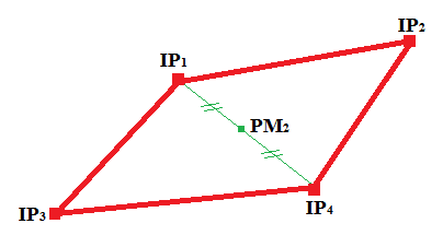
Figure 3.3.8.2-5: calculation in the reference coordinate system, of a middle point of the second type, located on a quadrangle face

Middle points of the second type verify the equation of intersection of a line with the following iso-zero:

\(\begin{array}{c}{\xi }_{{\mathit{PM}}_{2}}={\xi }_{M}+t\vec{v}\\ {\mathit{lsn}}^{h}\left({\xi }_{{\mathit{PM}}_{2}}\right)=0\end{array}\)

Depending on the location of the midpoint (either located between 2 intersection points, or located inside the quadrangle face on the iso-zero), we explained the exact coordinates of \({\xi }_{M}\) and \(\vec{v}\) in the reference element.

We solve the search for the zero in equation \({\mathit{lsn}}^{h}\left({\xi }_{M}+t\vec{v}\right)=0\) by a Newton as in paragraph § 2.2.3. In order to ensure that Newton’s algorithm « stays » respectively in face TRIA for a middle point of the second type located between two points of intersection and in the sub-element TETRA for a middle point of the second type located at the center of a quadrangle face, the Newton algorithm is strengthened by the Dekker method. If an iteration of Newton’s algorithm sends us outside the authorized search area, a dichotomy will be preferred to get closer to the solution. Indeed, sometimes equation \(\begin{array}{c}{\xi }_{{\mathit{PM}}_{2}}={\xi }_{M}+t\vec{v}\\ {\mathit{lsn}}^{h}\left({\xi }_{{\mathit{PM}}_{2}}\right)=0\end{array}\) has several solutions, but there is only one that is in the search side TRIA or in the search sub-element TETRA. This solution can be difficult to capture by Newton’s algorithm, especially when curve \(\mathit{lsn}=0\) has a significant curvature or « erases » an edge of face TRIA or a face of sub-element TETRA (see and).

Figure 3.3.8.2-6: existence of close solutions for the middle point of type 2 in a face TRIA

Figure 3.3.8.2-7: existence of close solutions for the middle point of type 2 located on a quadrangle face in a sub-element TETRA

Figure 3.3.8.2-8: limits of the « search space » in face TRIA for a middle point of the second type located between two intersection points

Figure 3.3.8.2-9: limits of the « search space » in sub-element TETRA for a middle point of the second type located at the center of a quadrangle face

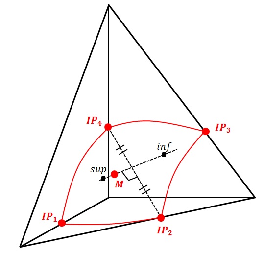
Newton-Raphson algorithm for calculating a midpoint located on the isozero of the level-set:

• • Newton-Raphson initialization: \({t}_{0}=0\)

  • Determination of the lower and upper limits \({t}_{\mathit{min}}\) and \({t}_{\mathit{max}}\) of the search space (see and)

• • • \({\xi }_{n}={t}_{n}\vec{v}+{\xi }_{M}\)

    • Calculating the function: \({\mathit{lsn}}^{h}({\xi }_{n})=\sum _{1⩽j⩽\mathit{nnop}}{\mathit{lsn}}_{j}{\Phi }_{j}({\xi }_{n})\)

• Calculation of the derivative: \({\mathit{dlsn}}^{h}({\xi }_{n})/\mathit{dt}=\sum _{1⩽j⩽\mathit{nnop}}{\mathit{lsn}}_{j}\nabla {\Phi }_{j}({\xi }_{n})\cdot \vec{v}\)

• Slope check: if \(∣{\mathit{dlsn}}^{h}({\xi }_{n})/\mathit{dt}∣<{10}^{-16}\) then exit with error code.

• • Calculating the increment: \({\Delta }_{n}=\frac{{\mathit{lsn}}^{h}({\xi }_{n})}{{\mathit{dlsn}}^{h}({\xi }_{n})/\mathit{dt}}\)

• • Calculation of the new position: \({t}_{n+1}={t}_{n}-{\Delta }_{n}\)

  • If \({t}_{n+1}\in [{t}_{\mathit{min}},{t}_{\mathit{max}}]\), then we continue, otherwise:

  • If \({t}_{n+1}>{t}_{\mathit{max}}\), then \({t}_{n+1}=\frac{{t}_{n}+{t}_{\mathit{max}}}{2}\)

  • If \({t}_{n+1}<{t}_{\mathit{min}}\), then \({t}_{n+1}=\frac{{t}_{n}+{t}_{\mathit{min}}}{2}\)

• • Criterion for stopping the increment: if \(∣{\Delta }_{n}∣<{10}^{-8}\) then end of the loop.

• Calculation of the reference coordinates of the intersection point: \({\xi }_{\infty }={t}_{\infty }\vec{v}+M\)

• • Verification of hypothesis \({\xi }_{\infty }\in \mathit{ELREFP}\): if \({\xi }_{\infty }\notin \mathit{ELREFP}\) then exit with error code.

• • Calculation of real coordinates by interpolation of geometric coordinates:

\(X({\xi }_{\infty })=\sum _{1⩽j⩽\mathit{nnop}}{X}^{j}{\Phi }_{j}({\xi }_{\infty })\)

For non-simplicial elements, there is a situation where the search for the middle point type 2 is useless in the authorized search space (between the \(\mathit{inf}\) and \(\text{sup}\) terminals). As indicated in paragraph § 3.3.1, sub-element cutting is based on a reduction of non-simplicial elements into simplicial elements (TRIA in 2D and TETRA in 3D). However, this reduction can lead to situations that make the search for type 2 midpoints impossible in the subdivision of non-simplistic elements. An example is shown in the figure on the left. We are looking for the middle point of type 2 between the intersection points \({\mathit{IP}}_{1}\) and \({\mathit{IP}}_{2}\). However, in the authorized search interval (between the limits \(\mathit{inf}\) and \(\text{sup}\)), the field of \(\mathit{lsn}\) has a constant sign. The Newton-Raphson algorithm is therefore unsuccessful. The internal diagonal edge is in fact intersected by the curve \(\mathit{lsn}=0\) even though the latter was detected as not cut because the value of the \(\mathit{lsn}\) at each of its 3 nodes is strictly of the same sign. But unlike an edge of the parent element, the \(\mathit{lsn}\) field along this inner edge depends on the value of \(\mathit{lsn}\) at each of the 8 nodes of the parent element QUAD8, and not only on the value of \(\mathit{lsn}\) at its 3 nodes. That’s why the \(\mathit{lsn}\) field changes signs along this inner edge. This difficulty can be circumvented by choosing another bijection for dividing the quadrangle into two triangles (confer). On the right, we use the other bijection to cut the quadrangle into two triangles in order to avoid a change in the sign of field \(\mathit{lsn}\) along the inner edge. The middle points of the second type \({M}_{1}\) and \({M}_{2}\) are then determined in the authorized intervals. So each time the search for a middle point of the second type in the interval \([\mathit{inf},\text{sup}]\) is unsuccessful within a simplicial element, the procedure for cutting the element is restarted by choosing a different bijection for the division into triangular (or tetrahedral in 3D) subcells. In the case where all the possible bijections would not have made it possible to provide a solution to this problem, a linear approximation of the curve \(\mathit{lsn}=0\) is then carried out, where the midpoint is chosen as being the middle of the segment \([{\mathit{IP}}_{1}{\mathit{IP}}_{2}]\) in the reference space.

Figure 3.3.8.2-10: Cases of aborting the search for a type 2 midpoint for non-simplicial elements.

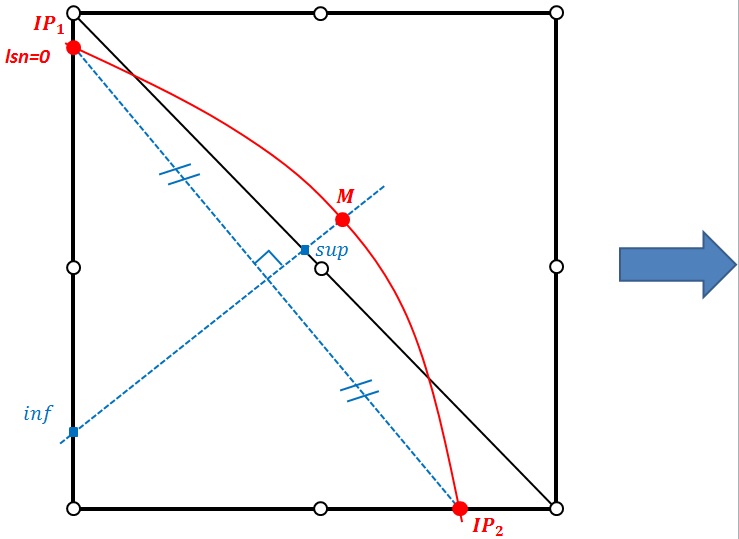
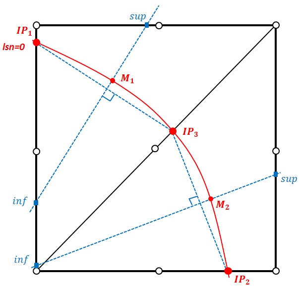
These cases are rare and only occur when the curvature of the interface is significant in relation to the size of the cells. By refining the mesh sufficiently, one is assured of not running into this problem.

• for a midpoint of the**third type**, located on a quadrangle face of a child polyhedron (pyramid or pentahedron), the virtual cutting edge connects the first intersection point \({\mathit{IP}}_{1}\) of the face and a vertex node of the tetrahedron \(B\) (see). Regarding the positioning of the midpoint on the quadrangle face:

• if the level-set is curved, we make the following choice: \({\xi }_{{\mathit{PM}}_{3}}={\xi }_{\mathit{Milieu}\left({\mathit{PM}}_{2}\text{-}D\right)}=\frac{{\xi }_{{\mathit{PM}}_{2}}+{\xi }_{D}}{2}\) so that the calculated midpoint does not come out of the quadrangle face.

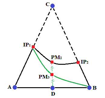
Figure 3.3.8.2-11: calculation in the reference frame, of a middle point of the third type for a curved iso-zero

Note on the curvature criterion

To judge the curvature of the LSN, the following procedure is performed. We first consider the midpoint \({\mathit{PM}}_{3}\) candidate as \({\xi }_{{\mathit{PM}}_{3}}={\xi }_{\mathit{Milieu}({\mathit{IP}}_{1}\text{-}B)}=\frac{{\xi }_{{\mathit{IP}}_{1}}+{\xi }_{B}}{2}\). We then calculate the sine of the angle between the vectors \(\vec{{\mathit{IP}}_{\mathrm{1,}}{\mathit{PM}}_{2}}\) and \(\vec{{\mathit{IP}}_{\mathrm{1,}}{\mathit{PM}}_{3}}\) , the plane being oriented with respect to the outgoing normal coming towards the reader. If negative, this midpoint will give rise to distorted elements , otherwise the two resulting TRIA will be healthy. In practice, it is considered that the LSN is too curved when the sine is less than 0.1. We then select \({\mathit{PM}}_{3}\) such as .

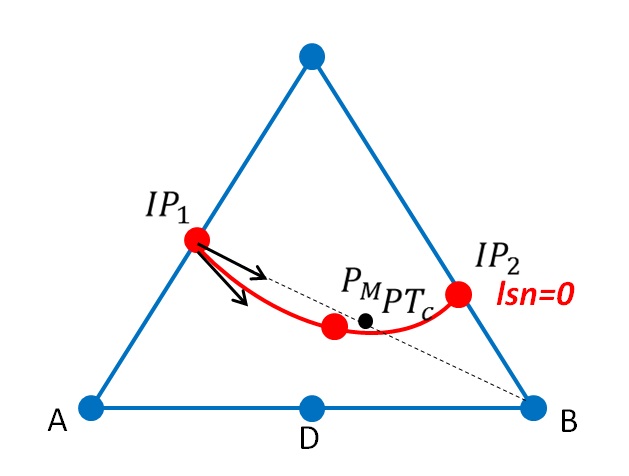
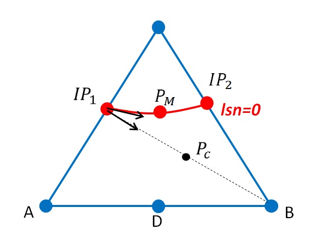
Figure 3.3.8.2-12: criterion for determining whether the LSN is considered to be curved: « curved » situation on the left and « healthy » on the right

Underdivision and discretization error

In the splitting procedure explained in § 3.3.8, the levet-set is always interpolated into the parent reference element. Therefore, the intersection points and midpoints positioned on the iso-zero, rigorously verify equation \({\mathit{lsn}}^{h}({\xi }^{\mathit{ELREFP}})=0\). Clearly, the algorithm for positioning the points on the iso-zero surface does not introduce any additional error compared to the interpolation error of the level-set.

In contrast, the geometric shape of the level-set is approximated by connecting the points calculated to form the border of the integration subdomains (see, where function \({\Phi }^{h}={\mathit{lsn}}^{h}({\xi }^{\mathit{ELREFP}})=0\) is a conic while the edge of the quadratic subcell that best coincides with this conic is parabolic).

Figure 3.3.8.2-13: Isozero approximation

3.4. Retrieving contact facets

3.4.1. XH elements

The recovery of contact facets is useful both for contact but also for applying mechanical pressure in the crack lips. To obtain these facets, we rely on the work of division into sub-elements described in § 3.3. In fact, the topology of the integration sub-elements already contains all the information on the contact facets, which are none other than the sides (in 2D) or the faces (in 3D) of the integration sub-elements that verify \(\mathit{lsn}=0\). It is therefore sufficient simply to go through the sides or faces of the integration sub-elements and to select those that are confused with the discontinuity (see). However, the summit nodes of the integration sub-elements, which are points of intersection, are identified by their connectivity between 1000 and 1999. In the case of an intersection point that is confused with a node of the parent element, we will have \(\mathit{lsn}=0\) directly for this node.

The facets that are recovered are linear 2D SEG2en, 2D quadratic SEG3en, 2D quadratic, TRIA3 in linear 3D, and TRIA6 in quadratic 3D. In order to retrieve the facets only once, the search is only performed on the sides or faces of the integration sub-elements such as \(\mathit{lsn}<0\).

Figure 3.4.1-1: integration sub-elements and contact facets in a QUAD8

In the example above, QUAD8 is divided into 6 TRIA6. The search for contact facets is performed on sub-elements 2, 3 and 4 that verify \(\mathit{lsn}<0\). We then get two SEG3 (in red).

Algorithm for recovering contact facets for XH elements:

• Loop over the \(\mathit{nse}\) sub-elements of the parent XH element

• If the sub-element checks for \(\mathit{lsn}<0\), then

• Loop on the vertex nodes on the current side or face

• if the connectivity of the node is between 1000 and 1999, it is a point of intersection with the discontinuity, it is selected.

• if the connectivity of the vertex node is strictly less than 1000, then it is a vertex node of the parent element, it is selected only if it verifies \(\mathit{lsn}=0\).

• End of the loop on the vertex nodes of the current face

• If all the vertex nodes on the current side or face have been selected, it is a contact facet, whose connectivity and the coordinates of its nodes are stored

• End of condition

• End of the loop on the \(\mathit{nse}\) sub-elements of the parent XH element

3.4.2. Elements XHT and XT

When the element is XHT or XT, additional work is required compared to the XH elements. Indeed, the sub-element cutting is done in accordance with \(\mathit{lsn}\), but not in accordance with \(\mathit{lst}\). The contact facets that are recovered therefore verify \(\mathit{lsn}=0\), but not necessarily \(\mathit{lst}<0\), because the elements XHT and XT are likely to contain the crack background. A redistribution in accordance with \(\mathit{lst}\) is then necessary.

Once the contact facets such as \(\mathit{lsn}=0\) have been obtained, they are cut again if necessary according to the curve \(\mathit{lst}=0\) (see)

To do this, exactly the same approach is used as when cutting the main elements into integration sub-elements (cutting in accordance with surface \(\mathit{lsn}=0\)). In the example below, the SEG2 on the right is cut along the \(\mathit{lst}=0\) curve.

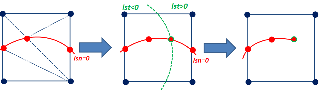
Figure 3.4.2-1: redistribution of facets at the crack bottom

3.4.3. Multi-Heaviside elements

For multi-cracked elements, the procedure is the same. In fact, sub-element cutting is carried out sequentially, crack after crack, so that the final integration sub-elements conform to each of the cracks (see). For each crack, the same process is then used as for the XH elements. However, for cracks where another crack connects, one does not necessarily perform a search for contact facets in elements such as \(\mathit{lsn}<0\). In order to ensure that the contact facets conform to the junction, the contact facets are searched on the side where the crack branches (see).

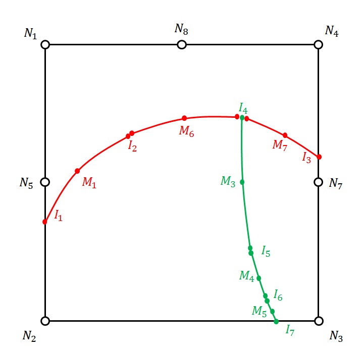
Figure 3.4.3-1: recovery of contact facets for a multi-cracked element. The facets of crack 1 are recovered from the side where crack 2 branches.

When several cracks connect to the same crack within an element, if all the connections are not made on the same side, there are generally no contact facets corresponding to each crack (see). The cutting algorithm then emits an alarm message that invites the user to refine the mesh so as to no longer have multiple junctions within the same element.

There is no redistribution required because multi-cracked elements cannot contain a crack background, they are interface elements only.

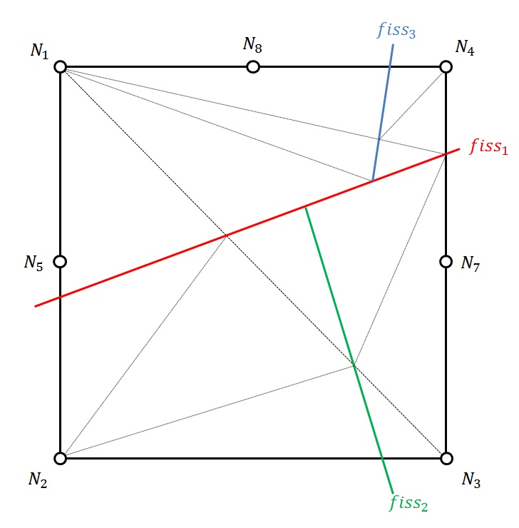
Figure 3.4.3-2: recovery of contact facets impossible for a multi-cracked element in which two cracks connect on either side of a first crack.

Algorithm for recovering contact facets for multi-cracked elements:

• Loop over the \(\mathit{nfiss}\) cracks that run through the element

\({\mathit{signe}}^{\mathit{ref}}=-1\)

If one or more cracks connect to \(\mathit{ifiss}\), we determine the sign corresponding to the side where the cracks branch into \({\mathit{signe}}^{\mathit{ref}}=\mathit{signe}(\mathit{côté})\). If the cracks do not all plug into the same side, the following alarm message is issued:

« Several cracks are connected on either side of the same crack within the same element. The recovery of contact facets that conform to each junction is likely to fail. Refine the mesh so that this situation does not happen again. »

• Loop over the \(\mathit{nse}\) sub-elements of the parent XH element

• If the sub-element checks for \({\mathit{signe}}^{\mathit{sous}\mathit{élément}}(\mathit{ifiss})={\mathit{signe}}^{\mathit{ref}}\), then

• Loop on the vertex nodes on the current side or face

• if the connectivity of the node is between 1000 and 1999, it is a point of intersection with one of the cracks, it is pre-selected. It is definitely selected if \(∣{\mathit{lsn}}^{\mathit{ifiss}}∣<\mathit{loncar}\ast {10}^{-8}\) with \(\mathit{loncar}\) being the characteristic length of the parent element. This part of the programming will evolve in order to get rid of this criterion. In fact, two nodes on the same side, with connectivity between 1000 and 1999, achieve the minimum of a single level and that is therefore easy to identify;

• if the connectivity of the vertex node is strictly less than 1000, then it is a vertex node of the parent element, it is selected only if it verifies \({\mathit{lsn}}^{\mathit{ifiss}}=0\).

• End of the loop on the vertex nodes of the current face

• If all the vertex nodes on the current side or face have been selected, it is a contact facet for crack \(\mathit{ifiss}\), whose connectivity and the coordinates of its nodes are stored

• End of condition

• End of the loop on the \(\mathit{nse}\) sub-elements of the parent XH element

End of the loop on the \(\mathit{nfiss}\) cracks that cross the element

---

3.4.4. Maximum number of facets retrieved

In the 2D case, you can have a maximum of 3 contact facets in a quadrangle (see).

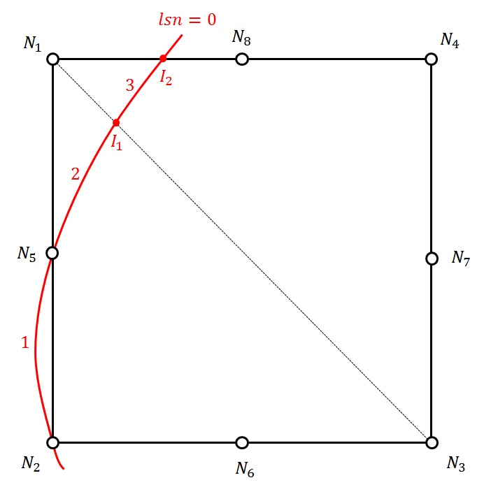
Figure 3.4.4.1-1: a quadrangle with 8 nodes and its 3 contact facets

In the 3D case, for a hexahedron, the maximum number of contact facets can be increased for a single crack by 18. This figure is in fact likely to be reached for an element that contains the crack base. When redividing triangular facets in accordance with \(\mathit{lst}\), some facets give rise to two facets (see), which explains why we can end up with nearly 18 facets.

Figure 3.4.4.2-1: redistribution of a triangular facet at the crack bottom

In the case of multiple cracks, the maximum number of contact facets per crack is higher than the maximum number of contact facets for an element crossed by a single crack. In fact, sequential cutting generates more sub-elements for each new crack and therefore more contact facets because the latter rely on the sub-elements. In 3D, for a hexahedron, the maximum number of contact facets per crack is set to 30. A 3D element crossed by 4 cracks can therefore have a total of \(30\ast 4=120\) facets. In 2D, the maximum number of contact facets per crack is set to 7. A 2D element crossed by 4 cracks can therefore have a total of \(4\ast 7=28\) facets.

3.5. Integrating stiffness

3.5.1. Integral of the mechanical stiffness term

The X- FEM approximation of the displacement field is written in vector form:

\(\left\{{u}^{h}\right\}=\left\{{\mathrm{\varphi }}_{i}\phantom{\rule{2em}{0ex}}{\mathrm{\varphi }}_{j}{H}_{j}\phantom{\rule{2em}{0ex}}{\mathrm{\varphi }}_{k}{F}^{1}\phantom{\rule{2em}{0ex}}{\mathrm{\varphi }}_{k}{F}^{2}\phantom{\rule{2em}{0ex}}{\mathrm{\varphi }}_{k}{F}^{3}\phantom{\rule{2em}{0ex}}{\mathrm{\varphi }}_{k}{F}^{4}\right\}\cdot \left\{\begin{array}{c}{a}_{i}\\ {b}_{j}\\ {c}_{k}^{1}\\ {c}_{k}^{2}\\ {c}_{k}^{3}\\ {c}_{k}^{4}\end{array}\right\}\)

Or again:

\(\left\{{u}^{h}\right\}=\left\{N\right\}\cdot \left\{u\right\}\)

where \(\left\{N\right\}\) is the vector of the enriched base of shape functions and \(\left\{u\right\}\) is the vector of the modal displacement ddls.

Deformations are written as:

\(\left\{\epsilon \right\}=\left[B\right]\cdot \left\{u\right\}\)

where \(\left[B\right]\) is the matrix of derivatives of form functions

\(\left[B\right]=\left\{{\left(\mathrm{\varphi }\right)}_{{i}^{\prime }}\phantom{\rule{2em}{0ex}}{\left({\mathrm{\varphi }}_{j}\right)}^{\prime }{H}_{j}\phantom{\rule{2em}{0ex}}{\left({\mathrm{\varphi }}_{k}\right)}^{\prime }{F}^{\alpha }+{\mathrm{\varphi }}_{k}{\left({F}^{\alpha }\right)}^{\prime }\right\},\phantom{\rule{2em}{0ex}}\alpha =\mathrm{1,4}\)

On a finite element X- FEM occupying a domain \({O}_{e}\), the expression for the elementary stiffness matrix is (according to the expression eq 3.1.4 of PTV):

\(\left[{K}_{e}\right]={\int }_{{\Omega }_{e}}{\left[B\right]}^{t}\left[D\right]\left[B\right]d{\Omega }_{e}\)

We subdivide the integral into a sum of integrals over the sub-elements:

\(\left[{K}_{e}\right]=\sum _{\text{sous-éléments}}{\int }_{{\Omega }_{\text{se}}}{\left[B\right]}^{t}\left[D\right]\left[B\right]d{\Omega }_{\text{se}}\)

Note in passing that the quantities to be integrated do not change, and always refer to the finite element X- FEM \({O}_{e}\) (called « parent element ») and not to the sub-elements \({O}_{\text{se}}\).

On each sub-element, the integrand is continuous. In fact, the sub-elements respect the discontinuity of the crack, so the function \({H}_{j}\left(x\right)\) is constant there, and the functions \({\phi }_{{i}^{\prime }}\), \({F}^{\alpha }\) and \({({F}^{\alpha })}^{\prime }\) are continuous.

3.5.2. Integral of the geometric rigidity term

When dealing with large rotations or large deformations, geometric rigidity must be taken into account. Geometric rigidity is also useful in the case of modal analysis.

In the case of large rotations, for example, the virtual work of the internal forces can be written on the initial configuration in the form:

\(\delta {\pi }_{\text{int}}={\int }_{\Omega }(S(E)\text{:}\delta {E}^{\text{}\ast \text{}})d\Omega\)

where \(E\) and \(S\) are the Green-Lagrange deformation and Piola-Kirchhoff stress vectors of the second kind respectively.

The iterative variation of virtual work is then written as:

\(\Delta \delta {\pi }_{\text{int}}={\int }_{\Omega }(\Delta S(E)\text{:}\delta {E}^{\text{}\ast \text{}}+S(E)\text{:}\Delta \delta {E}^{\text{}\ast \text{}})d\Omega\)

and using the fact that:

\([E]=\frac{1}{2}(\mathrm{Ñu}\text{+Ñ}{u}^{T}\text{+Ñ}{u}^{T}\mathrm{Ñu})\)

\([\Delta E]=\frac{1}{2}(\nabla \Delta u+\nabla \Delta {u}^{T}+\text{}\nabla \Delta {u}^{T}\nabla {u}^{T}+\text{}\nabla {u}^{T}\nabla \Delta u)\)

and:

\([\delta \Delta E]=\frac{1}{2}(\text{}\nabla \Delta {u}^{T}\nabla \delta u\text{}+\text{}\nabla \delta {u}^{T}\nabla \Delta u)\)

the variation in virtual work becomes:

\(\Delta \delta {\pi }_{\text{int}}={\int }_{\Omega }(\Delta S(E)\text{:}\delta {E}^{\text{}\ast \text{}}+\mathrm{tr}({\nabla }^{T}{u}^{\text{}\ast \text{}}\cdot S\cdot \nabla \mathrm{\delta u}))d\Omega\)

The integral on an element X- FEM of the second term of this equation which can be written (in 2D):

\({\int }_{{\Omega }_{e}}\mathrm{tr}({\nabla }^{T}{u}^{\text{}\ast \text{}}\cdot S\cdot \nabla \mathrm{\delta u})d{\Omega }_{\mathrm{se}}=\sum _{\text{se}}{\int }_{{\Omega }_{\mathrm{se}}}{\sum }_{m,n}{(\begin{array}{cccccc}{a}_{X}^{\text{}\ast \text{}}& {a}_{Y}^{\text{}\ast \text{}}& {b}_{X}^{\text{}\ast \text{}}& {b}_{Y}^{\text{}\ast \text{}}& {c}_{X}^{\alpha \text{}\ast \text{}}& {c}_{Y}^{\alpha \text{}\ast \text{}}\end{array})}_{m}\cdot {[{K}_{\mathrm{se}}^{\mathrm{geom}}]}_{m,n}\cdot {(\begin{array}{c}{\mathrm{\delta a}}_{X}\\ {\mathrm{\delta a}}_{Y}\\ {\mathrm{\delta b}}_{X}\\ {\mathrm{\delta b}}_{Y}\\ {\mathrm{\delta c}}_{X}^{\beta }\\ {\mathrm{\delta c}}_{Y}^{\beta }\end{array})}_{n}d{\Omega }_{\mathrm{se}}\)

shows the geometric rigidity matrix of the sub-element:

\({\mathrm{[}{K}_{\mathit{se}}^{\mathit{geom}}\mathrm{]}}_{m,n}\mathrm{=}(\begin{array}{cccccc}{\phi }_{,i}^{m}{S}_{\mathit{ij}}{\phi }_{,j}^{n}& 0& H{\phi }_{,i}^{m}{S}_{\mathit{ij}}{\phi }_{,j}^{n}& 0& {\phi }_{,i}^{m}{S}_{\mathit{ij}}({\phi }_{,j}^{n}{F}^{\beta }+{\phi }_{j}^{n}{F}_{,j}^{\beta })& 0\\ 0& {\phi }_{,i}^{m}{S}_{\mathit{ij}}{\phi }_{,j}^{n}& 0& H{\phi }_{,i}^{m}{S}_{\mathit{ij}}{\phi }_{,j}^{n}& 0& {\phi }_{,i}^{m}{S}_{\mathit{ij}}({\phi }_{,j}^{n}{F}^{\beta }+{\phi }_{j}^{n}{F}_{,j}^{\beta })\\ H{\phi }_{,i}^{m}{S}_{\mathit{ij}}{\phi }_{,j}^{n}& 0& {H}^{2}{\phi }_{,i}^{m}{S}_{\mathit{ij}}{\phi }_{,j}^{n}& 0& H{\phi }_{,i}^{m}{S}_{\mathit{ij}}({\phi }_{,j}^{n}{F}^{\beta }+{\phi }_{j}^{n}{F}_{,j}^{\beta })& 0\\ 0& H{\phi }_{,i}^{m}{S}_{\mathit{ij}}{\phi }_{,j}^{n}& 0& {H}^{2}{\phi }_{,i}^{m}{S}_{\mathit{ij}}{\phi }_{,j}^{n}& 0& H{\phi }_{,i}^{m}{S}_{\mathit{ij}}({\phi }_{,j}^{n}{F}^{\beta }+{\phi }_{j}^{n}{F}_{,j}^{\beta })\\ ({\phi }_{,i}^{m}{F}^{\alpha }+{\phi }_{i}^{m}{F}_{,i}^{\alpha }){S}_{\mathit{ij}}{\phi }_{,j}^{n}& 0& ({\phi }_{,i}^{m}{F}^{\alpha }+{\phi }_{i}^{m}{F}_{,i}^{\alpha }){S}_{\mathit{ij}}H{\phi }_{,j}^{n}& 0& ({\phi }_{,i}^{m}{F}^{\alpha }+{\phi }_{i}^{m}{F}_{,i}^{\alpha }){S}_{\mathit{ij}}({\phi }_{,j}^{n}{F}^{\beta }+{\phi }_{j}^{n}{F}_{,j}^{\beta })& 0\\ 0& ({\phi }_{,i}^{m}{F}^{\alpha }+{\phi }_{i}^{m}{F}_{,i}^{\alpha }){S}_{\mathit{ij}}{\phi }_{,j}^{n}& 0& ({\phi }_{,i}^{m}{F}^{\alpha }+{\phi }_{i}^{m}{F}_{,i}^{\alpha }){S}_{\mathit{ij}}H{\phi }_{,j}^{n}& 0& ({\phi }_{,i}^{m}{F}^{\alpha }+{\phi }_{i}^{m}{F}_{,i}^{\alpha }){S}_{\mathit{ij}}({\phi }_{,j}^{n}{F}^{\beta }+{\phi }_{j}^{n}{F}_{,j}^{\beta })\end{array})\)

where \(n\) and \(m\) correspond to the node numbers in the parent element.

3.5.3. Calculation of derivatives of singular functions:

We are looking for the derivatives of singular functions with respect to global coordinates \((x,y,z)\). Singular functions are given according to polar coordinates \((r,\theta )\).

Derivatives of singular functions in the polar base \((r,\theta )\):

\(\left[\begin{array}{cc}\frac{\mathrm{\partial }{F}^{1}}{\mathrm{\partial }r}& \frac{\mathrm{\partial }{F}^{1}}{\mathrm{\partial }\theta }\\ \frac{\mathrm{\partial }{F}^{2}}{\mathrm{\partial }r}& \frac{\mathrm{\partial }{F}^{2}}{\mathrm{\partial }\theta }\\ \frac{\mathrm{\partial }{F}^{3}}{\mathrm{\partial }r}& \frac{\mathrm{\partial }{F}^{3}}{\mathrm{\partial }\theta }\\ \frac{\mathrm{\partial }{F}^{4}}{\mathrm{\partial }r}& \frac{\mathrm{\partial }{F}^{4}}{\mathrm{\partial }\theta }\end{array}\right]\mathrm{=}\left[\begin{array}{cc}\frac{1}{2\sqrt{r}}\text{sin}\frac{\theta }{2}& \frac{\sqrt{r}}{2}\text{cos}\frac{\theta }{2}\\ \frac{1}{2\sqrt{r}}\text{cos}\frac{\theta }{2}& \mathrm{-}\frac{\sqrt{r}}{2}\text{sin}\frac{\theta }{2}\\ \frac{1}{2\sqrt{r}}\text{sin}\frac{\theta }{2}\text{sin}\theta & \frac{\sqrt{r}}{2}\text{cos}\frac{\theta }{2}\text{sin}\theta +\sqrt{r}\text{sin}\frac{\theta }{2}\text{cos}\theta \\ \frac{1}{2\sqrt{r}}\text{cos}\frac{\theta }{2}\text{sin}\theta & \mathrm{-}\frac{\sqrt{r}}{2}\text{sin}\frac{\theta }{2}\text{sin}\theta +\sqrt{r}\text{cos}\frac{\theta }{2}\text{cos}\theta \end{array}\right]\)

Derivatives of singular functions in the local base \(\left\{{e}_{1},{e}_{2},{e}_{3}\right\}\):

\(\left[\begin{array}{ccc}\frac{\partial {F}^{1}}{\partial {x}_{1}}& \frac{\partial {F}^{1}}{\partial {x}_{2}}& \frac{\partial {F}^{1}}{\partial {x}_{3}}\\ \frac{\partial {F}^{2}}{\partial {x}_{1}}& \frac{\partial {F}^{2}}{\partial {x}_{2}}& \frac{\partial {F}^{2}}{\partial {x}_{3}}\\ \frac{\partial {F}^{3}}{\partial {x}_{1}}& \frac{\partial {F}^{3}}{\partial {x}_{2}}& \frac{\partial {F}^{3}}{\partial {x}_{3}}\\ \frac{\partial {F}^{4}}{\partial {x}_{1}}& \frac{\partial {F}^{4}}{\partial {x}_{2}}& \frac{\partial {F}^{4}}{\partial {x}_{3}}\end{array}\right]=\left[\begin{array}{cc}\frac{\partial {F}^{1}}{\partial r}& \frac{\partial {F}^{1}}{\partial \theta }\\ \frac{\partial {F}^{2}}{\partial {x}_{1}}& \frac{\partial {F}^{2}}{\partial \theta }\\ \frac{\partial {F}^{3}}{\partial {x}_{1}}& \frac{\partial {F}^{3}}{\partial \theta }\\ \frac{\partial {F}^{4}}{\partial {x}_{1}}& \frac{\partial {F}^{4}}{\partial \theta }\end{array}\right]\left[\begin{array}{ccc}\text{cos}\theta & \text{sin}\theta & 0\\ \frac{-\text{sin}\theta }{r}& \frac{\text{cos}\theta }{r}& 0\end{array}\right]\)

Derivatives of singular functions in the global base \(\left\{{E}_{1},{E}_{2},{E}_{3}\right\}\):

\(\left[\begin{array}{ccc}\frac{\partial {F}^{1}}{\partial x}& \frac{\partial {F}^{1}}{\partial y}& \frac{\partial {F}^{1}}{\partial z}\\ \frac{\partial {F}^{2}}{\partial x}& \frac{\partial {F}^{2}}{\partial y}& \frac{\partial {F}^{2}}{\partial z}\\ \frac{\partial {F}^{3}}{\partial x}& \frac{\partial {F}^{3}}{\partial y}& \frac{\partial {F}^{3}}{\partial z}\\ \frac{\partial {F}^{4}}{\partial x}& \frac{\partial {F}^{4}}{\partial y}& \frac{\partial {F}^{4}}{\partial z}\end{array}\right]=\left[\begin{array}{ccc}\frac{\partial {F}^{1}}{\partial {x}_{1}}& \frac{\partial {F}^{1}}{\partial {x}_{2}}& \frac{\partial {F}^{1}}{\partial {x}_{3}}\\ \frac{\partial {F}^{2}}{\partial {x}_{1}}& \frac{\partial {F}^{2}}{\partial {x}_{2}}& \frac{\partial {F}^{2}}{\partial {x}_{3}}\\ \frac{\partial {F}^{3}}{\partial {x}_{1}}& \frac{\partial {F}^{3}}{\partial {x}_{2}}& \frac{\partial {F}^{3}}{\partial {x}_{3}}\\ \frac{\partial {F}^{4}}{\partial {x}_{1}}& \frac{\partial {F}^{4}}{\partial {x}_{2}}& \frac{\partial {F}^{4}}{\partial {x}_{3}}\end{array}\right]{\left[P\right]}_{\text{Ee}}^{-1}\)

where \({\left[P\right]}_{\text{Ee}}\) is the transition matrix from the global database to the local base, such as

\(\begin{array}{cccc}& & \begin{array}{ccc}\phantom{\text{[}}{e}_{1}& {e}_{2}& {e}_{3}\phantom{\text{]}}\end{array}& \\ {[P]}_{\mathrm{Ee}}& \text{=}& \left[\begin{array}{ccc}\times & \times & \times \\ \times & \times & \times \\ \times & \times & \times \end{array}\right]& \begin{array}{c}{E}_{1}\\ {E}_{2}\\ {E}_{3}\end{array}\end{array}\)

To express a quantity in the global base, we produce the product of this matrix by the quantity expressed in the local base, i.e.

\({X}_{E}={\left[P\right]}_{\text{Ee}}{X}_{e}\)

Since this matrix is orthonormal, its inverse is easily obtained:

\({\left[P\right]}_{\text{Ee}}^{-1}={\left[P\right]}_{\text{Ee}}^{t}\)

3.5.4. Integration diagrams

For non-singular terms (classical terms and Heaviside enrichment), the functions to be integrated are polynomials. Numerical integration by a Gauss-Legrendre diagram on each subtetrahedron is then well suited. Let \(\text{npg}\) be the number of Gauss points. These points have coordinates in the reference subtetrahedron \(({s}_{g},{t}_{g},{u}_{g})\) and the associated weight is noted \({w}_{g}\). Let \(J\) be the Jacobian of the subtetrahedron transformation \(\to\) subtetrahedron of reference. Its determinant is constant per sub-element. The classic procedure is written as:

\({\int }_{{\Omega }_{\mathrm{se}}}fd{\Omega }_{\mathrm{se}}={\int }_{{\Omega }_{\mathrm{se}}^{\mathrm{ref}}}f\mid \text{det}(J)\mid d{\Omega }_{\mathrm{se}}\approx \sum _{g=1}^{\text{npg}}f({s}_{g},{t}_{g},{u}_{g}){w}_{g}\mid \text{det}(J)\mid\)

Since the function \(f\) is only known in the coordinate system linked to the parent reference element, it is necessary to express the coordinates of the Gauss point \(({s}_{g},{t}_{g},{u}_{g})\) in this coordinate system [bib 33]. First, we transport them into the real coordinate system (simple use of subtetrahedron shape functions), then we transport them into the coordinate system linked to the parent reference element (resolution of non-linear equations by the Newton-Raphson algorithm):

\(({s}_{g},{t}_{g},{u}_{g})\stackrel{{t}_{1}}{\to }({x}_{g},{y}_{g},{z}_{g})\stackrel{{t}_{2}}{\to }({\xi }_{g},{\eta }_{g},{\zeta }_{g})\)

Note:

Indeed, you should write \({\int }_{{\Omega }_{\text{se}}^{\text{ref}}}f°{t}_{2}°{t}_{1}({s}_{g},{t}_{g},{u}_{g})\mid \text{det}(J)\mid d{\Omega }_{\text{se}}\) instead. The transformation \({t}_{1}\) is linear. On the other hand, the transformation \({t}_{2}\) is non-linear. It is the opposite of a linear transformation. It is a combination of rational fractions and square roots with several variables. As a result, we do not know the effect of \(f°{t}_{2}°{t}_{1}\) on.*the maximum order of monomials in the general case. On the other hand, for a real element with parallel edges (diamond in 2D),* \({t}_{2}\) being linear, we consider that \(f°{t}_{2}°{t}_{1}({s}_{g},{t}_{g},{u}_{g})\) to be monomials in \(({s}_{g},{t}_{g},{u}_{g})\) of the same order as those defined on the parent reference element.

The shape functions of iso-parametric elements are monomials of type \({\xi }^{i}{\eta }^{j}{\zeta }^{k}\) with \(i+j+k\le p\) (see Tableau 3.5.4.1-1). The derivatives of the form functions are then monomials of the same type with \(i+j+k\mathrm{\le }p\mathrm{-}1\). The quantities to be integrated are therefore monomials of order \(m={(p-1)}^{2}\). We refer to [bib 34] to determine the appropriate diagram allowing exact integration [3] of all terms. For elements with non-parallel edges, integration will then be approximated.

Parent element	\(p\)	\(m={(p-1)}^{2}\)	\(\text{npg}\)
hexahedron	3	4	15
pentahedron	2	1	1
tetrahedron	1	0	1

Table 3.5.4.1-1 : Integration schemes by parent element type

Gauss-Legendre numerical integration schemes were designed for the integration of polynomials. However, the presence of monomials in \(1/\sqrt{r}\) resulting from the enrichment with asymptotic fields leads to a very slow convergence of the precision of these schemes: a considerable number of Gauss points is then necessary to obtain an acceptable error. When the singularity is on the border of the integration domain, changes of well-chosen successive variables make it possible to reduce to the integration into a unitary domain of a non-singular, polynomial (or quasi-polynomial) function, on which a classical Gauss-Legendre integration proves to be effective and rapidly convergent [bib 28]. A dozen Gauss points in each direction are enough to reach the limits of the numerical precision of a computer. When the singularity is not on the border, it is appropriate to divide the domain into sub-domains, so that the singularity is located on the borders of the sub-domains. Despite very satisfactory results in terms of convergence of the relative integration error on each term [bib 28], the implementation effort to be made for 3D structures seems considerable to us [bib 35]. Especially since the difference in global errors (after resolution) between a classical integration with a fairly high but reasonable number of Gauss points and a modified singular integration is not really significant

For the moment, we have implemented the same classical Gauss-Legendre scheme as that used for the integration of non-singular terms.

3.6. Integration of the second surface members

3.6.1. Integral of the second member of the surface forces

The second members due to surface forces can be written in a discretized manner:

\({\int }_{{\Gamma }^{t}}t\cdot {u}^{\ast }{\mathrm{d\Gamma }}^{t}\)

the discretized surface \({\Gamma }^{t}\) corresponds to the faces of the 3D elements. A possible sub-division for its 2D faces is that corresponding to the trace of the sub-division of the 3D elements. In Aster, we choose to take the generic 2D sub-division, corresponding to the one described in paragraph [§ 3.3.7].

Just as for the integration of stiffness, you need to determine the coordinates of the Gauss points of the reference sub-triangle in the parent reference element

Consider the Gauss point with coordinates \(({s}_{g},{t}_{g})\) in the reference sub-triangle. The problem is that the calculation environment is 3D, so we create a real 2D coordinate system local to each sub-triangle i.e. sub-triangle \(\text{ABC}\), normal \(n=\frac{\overrightarrow{\text{AB}}\wedge \overrightarrow{\text{AC}}}{\parallel \overrightarrow{\text{AB}}\wedge \overrightarrow{\text{AC}}\parallel }\). The local base is written as:

\({x}_{l}=\frac{\overrightarrow{\text{AB}}}{\parallel \overrightarrow{\text{AB}}\parallel },{y}_{l}=n\wedge {x}_{l}\).

The local coordinates of the Gauss point then are:

\(({x}_{g}{y}_{g})=(\sum _{i=1}^{3}{\psi }_{i}({s}_{g},{t}_{g}){x}^{i},\sum _{i=1}^{3}{\psi }_{i}({s}_{g},{t}_{g}){y}^{i})\)

where \({\psi }_{i}\) are the shape functions of the sub-triangles and \(({x}^{i},{y}^{i})\) are the coordinates of the vertices of the sub-triangle in the local 2D coordinate system \(({x}_{l},{y}_{l})\).

As for the integration of stiffness terms, it is now necessary to use a Newton-Raphson method to determine the coordinates of the Gauss point in the reference frame of the parent element (face element). For this, all the real coordinates are expressed in the real 2D local coordinate system.

3.6.2. Integral of the second limb of the surface forces on the lips of the crack

The second members due to the surface forces on the lips of the crack are written discretely:

\({\int }_{{\Gamma }_{c}}g\cdot {u}^{\ast }\mathrm{d\Gamma }\)

Integration takes place on both sides of the divide (\({\Gamma }_{c}={\Gamma }^{1}+{\Gamma }^{2}\)), with the convention:

• lip \({\Gamma }^{1}\) is such that the Heaviside function is negative and the polar angle is \(-\pi\),

• lip \({\Gamma }^{2}\) is such that the Heaviside function is positive and the polar angle is \(\pi\),

Note:

Since the norms outside the lips are opposite, the surface forces equivalent to the pressure imposed have opposite signs.

The integration of the second limb due to the forces applied to the lips takes place on the facets of the lips, thanks to the data of the objects corresponding to the discretization of the lips into triangular facets (see [§4.3 dans R5.03.54]). These objects were originally created to take contact into account.

For 2D elements, options CHAR_MECA_PRES_R, CHAR_MECA_PRES_F, CHAR_MECA_PCISA_R, and CHAR_MECA_CISA_F allow mechanical forces of distributed pressure and shear to be applied to the contact facets. Only options CHAR_MECA_PRES_R and CHAR_MECA_PRES_F are currently programmed for 3D elements, which means that it is not possible to apply shear forces to the lips.

In multi-cracking, it is possible to have different surface forces on different cracks.

The figure below () illustrates digital surface integration on the contact facets of a quadrangle. At each Gauss point of the facet, a normal unit vector and a tangent unit vector are determined solely using the topology of the contact facets.

Figure 3.6.2-1: surface integration on the facets of a quadrangle

In 3D, a normal unitary vector is determined in the same way at each Gauss point only from the topology of the contact facets. It is possible to create an orthonormal base at each Gauss point by completing this normal vector with two unit vectors tangent to the discontinuity and orthogonal to each other.

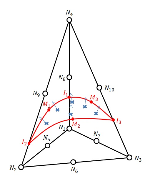
Figure 3.6.2-2: surface integration on the facets of a tetrahedron.

[1]

For a non-linear material, nothing changes in the formulation presented here. Only the calculation of stresses based on deformations and internal variables changes, which is transparent in this document.

[2]

For non-linear laws of behavior, this choice is retained, although this basis does not allow us to find the exact solution of the problem.

[3]

An integration maintaining the finite element approximation order would in fact be sufficient