1. Introduction

The incidents that occurred on concrete dams (Bouzey 1895, Gleno 1895, Gleno 1923, Malpasset 1959), as well as the results of auscultation, have shown that their stability, and therefore their safety, depends very largely on the hydromechanical behavior of the weakest areas of the valley-dam complex. Located at the level of discontinuities in the structure and in the rock, these weak points are mainly the faults in the support areas, the reinforcements of concrete in the dam, the concrete-rock contact of the foundation and the joints between the pillars of the dam. The mechanical behavior of these risk areas is highly non-linear, but thanks to their surface nature, industrial studies on major structures are complex but feasible. In addition to these difficulties, the method of construction of dams, the cleaving/sawing techniques used and its multiple drainage points make them structures whose modeling by finite elements is all the more complex in a conventional calculation code.

The three laws of behavior described in this document make it possible to take into account the main non-linearities of the behavior of structures: the phase of crack opening (JOINT_MECA_RUPT/ENDO) and the phase of sliding of its lips (JOINT_MECA_FROT/ENDO). Law JOINT_MECA_ENDO is the most complete law: it is capable of representing the evolution of the joint condition by combining the two phenomena of rupture (thanks to the damage variable) and friction (thanks to the plasticity variable).

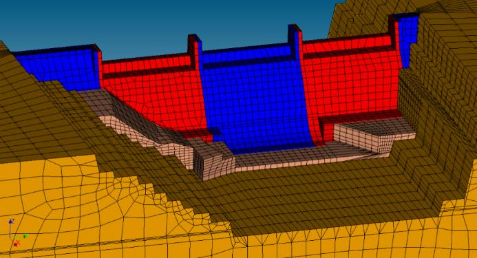
Figure 1-1: Dam under construction	Figure 1-2: Visualization of construction plots

1.1. Joints — weak links in the work

As mentioned earlier, dam joints have a varied origin (Figure). In general, the joint can be imagined as a rough discontinuity possibly reinforced by a filling material.

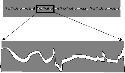
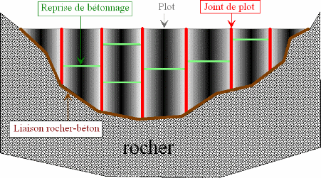
Figure 1.1-1: Physical joint image	Figure 1.1-2: Different types of dam joints

Coulomb’s law of friction, which uses only one parameter (coefficient of friction), captures only a tiny part of the very complex mechanical behavior of such a structure. In fact, apart from friction, the joint exhibits the following important phenomena: the loss of tensile strength, the elastic behavior at very low displacement, the gradual disappearance of the peak of shear stress for a cyclic loading. The relevance of these phenomena depends strongly on the physical state of the joint, in particular on its level of roughness, on the average size of the asperities, on the mechanical properties of the filling materials and on the rock matrix. Standard mechanical parameters such as Young’s modulus, Poisson’s ratio, or even the friction coefficient all influence joint behavior, but are not the only steps to be identified to capture the phenomena described above. The complete modeling of the joint therefore requires the introduction of a law depending on numerous parameters. Since the implementation of such a law in an implicit calculation code is a major technical challenge, we propose simpler laws, depending on few parameters but which nevertheless make it possible to capture the essential behavior of the joint under most current conditions of use. The latter are called JOINT_MECA_RUPT, JOINT_MECA_FROT and JOINT_MECA_ENDO. They make it possible to model the behavior of the joints found between the pillars of an arch dam and/or at the interface between the gravity dam and its foundation. We give a brief description of them below, before detailing them in the parts that follow.

1.2. Laws of mechanical behavior (without hydro coupling)

1.2.1. Breaking behavior JOINT_MECA_RUPT

Law JOINT_MECA_RUPTest is a softening elastic law, whose normal behavior is based on the cohesive formulation of the break. It opens up the possibility of modeling breakage in mode I (traction) and takes into account the coupling between normal opening and tangential stiffness. This law captures well the behavior of real joints at low displacements, as long as the sliding regime is not reached.

To identify the regimes in which it is applicable, we can use the physical image of the joint (Figure). These are two rough interfaces possibly containing a filling material between its lips; this can be either clay, or rock elements for the cracks between the dam and the foundation, or key grout for the joints of studs. Stress on the crack first involves the properties of the filling material and the geometry of the asperities that define the behavior of the structure at low displacements. As long as the filling material is not damaged or the asperities are not broken, the behavior of the joint remains elastic both when opened and when sheared. However, the parameters of normal and tangential stiffness, noted \({K}_{n}\) and \({K}_{t}\), are not equivalent, because they involve two distinct physical phenomena. The first is mainly related to the stiffness of the filling material, the second depends more on the flexural stiffness of the asperities. The joint has a tensile strength, noted \({\mathrm{\sigma }}_{\mathit{max}}\), which can be linked to the filling materials, but also to the transverse friction between the asperities of the two lips of the crack. The tensile strength is often quite low, not exceeding that of concrete \({\mathrm{\sigma }}_{\mathit{max}}\ll 1\mathit{MPa}\). As a first approximation, the normal stiffness can be estimated from Young’s modulus of the filling material \(E\) and the joint thickness \(e\), which gives \({K}_{n}=E/e\simeq 10\mathit{GPa}/1\mathit{cm}={10}^{12}\mathit{Pa}/m\). For sufficiently thick joints, the elastic behavior is isotropic and the tangential stiffness can be taken to be close to normal stiffness \({K}_{t}\simeq {K}_{n}\).

The rupture of the joint occurs gradually. In fact, the joint is first damaged by partially reducing its stiffness before breaking completely. To quantify this phenomenon we introduce a dimensionless breaking penalty parameter \({P}_{\mathit{rupt}}\), which represents a relative opening in softening compared to the elastic opening. For low \({P}_{\mathrm{rupt}}\) values, the break is sudden. For large values \({P}_{\mathit{rupt}}\gg 1\) the transition is more gradual, but this significantly increases the initial dissipation energy. Details of this behavior will be presented in the parts that follow. In practice, the value is taken close to \({P}_{\mathit{rupt}}\simeq 1\), which introduces the significant softening phase without straying too far from the abrupt breaking behavior.

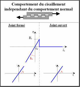
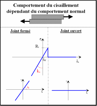
Figure 1.2-1: Normal and tangential behavior for extreme joint profiles: smooth joint on the right \(\alpha =0\), and infinitely rough joint \(\mathrm{\alpha }=2\) on the left

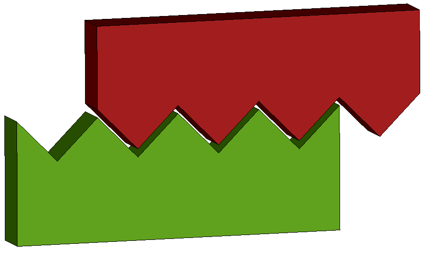
In order to model the different types of profiles of dam stud joints (represented in the Figure above), we introduce an additional parameter \(\alpha \mathrm{\in }\mathrm{[}\mathrm{0,2}\mathrm{]}\) into the user interface. This links the normal opening of the joint with the decrease in its tangential stiffness. Physically it reflects the depth of the asperities and varies continuously between \(0\) and \(2\). The value \(\mathrm{\alpha }=0\) corresponds to the smooth interface without asperities (the tangential stiffness drops to zero as soon as the joint is opened normally, see Figure on the right). The value \(\mathrm{\alpha }=2\) represents another extreme case, where the interface is very rough with an infinite depth of asperities, equivalent to the profile of a crenellated stud joint (Figure on the left). In this case, the tangential stiffness is not affected by the normal opening. The default value is set to \(1\), which represents an intermediate situation.

Figure 1.2-2: Realistic joint profile corresponding to intermediate roughness \(\mathrm{\alpha }=1\)

1.2.2. Sliding behavior JOINT_MECA_FROT

If you put more stress on the joint with pure shear, it will end up sliding with a certain coefficient of friction. Before moving into this plastic regime, a peak in the frictional force is experimentally observed. This phenomenon is linked to the fact that in order to be able to slide, the asperities must come out of their depressed position (dilatance). During this phase, the rubbing contacts are not necessarily parallel to the surface of the lips, which increases the effective friction coefficient. This « exit » procedure is accompanied in addition by an increase in the normal displacement of the joint. If this cycle is repeated several times, the stress peak subsides and disappears completely. It should be noted that the deeper the asperities, the greater the friction peak. In the case limiting even to the normal non-zero opening, the joint may reveal the elastic behavior in tangential slides (this case is treated by JOINT_MECA_RUPT with \(\alpha =2\)).

Law JOINT_MECA_FROT does not take into account all the complexity of sliding and in particular the peak, it only represents the ultimate sliding phenomenon, characterized by the only the coefficient of friction \(\mu\) and the adhesion \(c\) . The latter is linked to the tensile strength \({R}_{t}=c/\mathrm{\mu }\). The loss of tensile strength is not modelled by this law. As the load surface is assumed to be fixed once the peak of the cone is reached under tension, the evolution in perfect plasticity continues with the normal stress locked at the value of \({R}_{t}\). This behavior is clearly not a physical step for the fragile filling material and can only be considered as an approximation of the actual behavior. Law JOINT_MECA_FROT is written in elastoplastic formalism with the elastic phase identical to that of law JOINT_MECA_RUPT .

Figure 1.2-3: Typical tangential behavior: shear stress and normal opening as a function of tangential opening (measurements TEGG/EDF)

Figure 1.2-4: Load surface for law JOINT_MECA_FROT is a cone of revolution around the normal stress axis. It remains fixed during evolution.

Coupling behavior: breakage and friction JOINT_MECA_ENDO

The first two laws JOINT_MECA_RUPT/FROT are very basic and they only reproduce one and only one phenomenon at a time, either breaking or sliding. Each of the laws can be used in various parts of the book according to the local solicitation defined prior to the study. The advantage of such an approach lies in the simplicity of the laws used, since they depend only on a small number of parameters. However, in many situations, local change cannot be defined prior to the study, see cases where certain areas of the structure are stressed both when breaking and sliding.

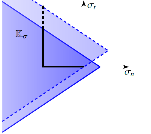
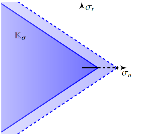
Law JOINT_MECA_ENDOa was introduced in order to deal with this type of situation, it combines the phenomena of rupture and sliding. As for law JOINT_MECA_FROTc “is an elastoplastic law with the conical load surface, but kinematic work hardening is introduced in addition, whose damaging nature makes it possible to represent softening both in tension and in shear. This is easily illustrated by the representation of the evolution of the load surface in the stress domain. The movement generated by the activation of the kinematic work hardening of the load surface spreads the elastic zone: the stress increases initially by following the loading direction. However, thanks to the damaging nature of the coupling, the amplitude of the work hardening decreases and the surface returns to its initial position for the final loads (completely damaged). This makes it possible to represent the peaks of tensile strength as well as that of sliding.

Figure 1.2-5: Movement generated by the kinematic work hardening of the load surface for law JOINT_MECA_ENDO, for normal loading (left) for shear (right)

1.3. Hydromechanical coupling

To assess the stability of dams, it is important to be able to model the propagation of sub-pressures between the rock and the dam foundation. Two possibilities are offered to the user. First, an underpressure profile can be imposed, as a load input parameter. This simple possibility makes it possible to study the stability of the dam for conservative hydraulic loading (the least favorable). On the other hand, the speed of the calculation has a significant advantage. It is thus possible to test an extreme hydraulic profile without spending more time than in pure mechanical calculation. In addition, this feature makes it possible to perform a hydromechanical chaining calculation. This consists in starting with a mechanical calculation with an initial state of pressure in the joints. Depending on the damage to the latter, the pressure profile (whose shape is given a priori) is updated. Once the pressure is changed, the mechanical condition of the joints changes again, which can cause some of them to break. The fluid then spreads more easily and the pressure profile changes again. This process is linked through a fixed point loop in the control file in order to obtain converged mechanical and hydraulic states.

Figure 1.3-1: Schematic representation of flow through the joint

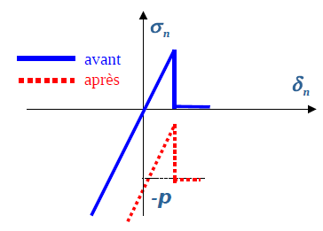
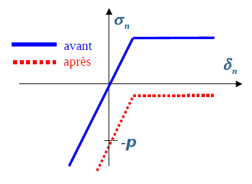
Figure 1.3-2: Taking hydrostatic pressure into account. Normal behavior relationship lag for law JOINT_MECA_RUPT (left) and law JOINT_MECA_FROT (right)

From the theoretical point of view, the introduction of fluid into the joint changes the normal mechanical stress \({\sigma }_{n}\to {\sigma }_{n}-p\) (Terzaghi’s law). In practice, the law of behavior in question is offset downwards according to the pressure value \(p\) at each integration point (cf. Figure 3.7).

These laws also accept coupled hydromechanical modeling, called xxx_ JOINT_HYME. The difference between the model with chaining hydromechanics (presented above) relates to the more precise consideration of the action of mechanics on hydraulics. In fact, in the chained model the profile is given a priori. In the coupled model, the opening of the joint changes the fluid flow law; the pressure profile is an unknown part of the problem. During hydromechanical coupling, to model the flow, the mechanical law is enriched by taking into account the cubic Poiseuille flow, which is regulated for very small crack openings. Thus, the pressure profile is no longer imposed, but calculated during the simulation. In addition to the standard mechanical equation, the following flow equation is solved simultaneously:

(1.1)\[ \ text {div}\ overrightarrow {w} =0;\ overrightarrow {w} =\ frac {\ rho} {12\ stackrel {} {\ mu}} {\ mu}} {\ delta}}} {\ delta}} _ {n} _ {n} _ {n}} ^ {3}\ overrightarrow {\nabla} p\]

where \(\overrightarrow{w}\) corresponds to the hydraulic flow, \({\delta }_{n}\) is the normal joint opening, and finally \(\rho\) and \(\stackrel{̄}{\mu }\) designate respectively the density and the dynamic viscosity of the fluid.

Note: Hydromechanical modeling is available for all JOINT_MECA_RUPT/FROT/ENDO behavior laws.

1.4. Claving procedure

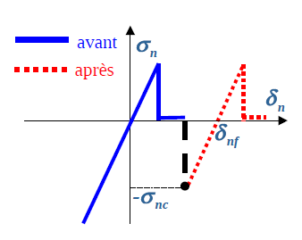
Figure 1.4-1: Illustration of the claving procedure Cleavage is a key step during the construction of an arch dam. It results in the injection of concrete grout under pressure between the dam blocks. It is therefore important to be able to model this process correctly. In practice, concrete casting is divided into several stages where the concrete is injected at different locations and at various pressures. From a mechanical point of view, claving is interpreted by compressing the lips of a keyed joint up to \({\sigma }_{n}=-{\sigma }_{\mathit{nc}}\) (pressure of the injected concrete, keyword PRES_CLAVAGE).

This option is directly included in the parameters of the law of behavior. Physically, claving is accompanied by a process of solidification of the injected grout; the procedure is modelled by modifying the thickness of the joints concerned. If the joint is initially strongly compressed, the claving does not influence it. On the other hand, if the joint is open or not sufficiently compressed (\({\sigma }_{n}>-{\sigma }_{\mathit{nc}}\)), the claving will result in the change of the thickness parameter of the joint noted \({\delta }_{\mathit{nf}}\). And, therefore, of a translation of the normal constraint.

The normal behavior of the joint after claving can be changed. Thus, the tensile strength can be restored (Figure) either partially or completely depending on the damage to the joints prior to the claving procedure. The procedure implemented consists in not restoring it, it keeps its current value.

Note: Clavage modeling is currently only available for basic laws JOINT_MECA_RUPT/FROT .Given the current numerical implementation, sawing and keying phenomena cannot be chained to the same joint.

1.5. Sawing procedure

It has been shown by in situ tests that the concrete of certain hydraulic structures in France has suffered damage due to the unknown alkali-aggregate chemical reaction at the time of the massive construction of dams before the war. The most notable example is the Chambon dam located on the Romanche, which after 80 years of existence was a victim of the phenomenon of concrete disease (RAG), so every fifteen years it must undergo special treatment. Microsawing operations on the structure make it possible to extend its lifespan. As the name suggests, this procedure consists of sawing the dam in order to release the compression stresses, which have developed over time. It is therefore important to be able to model this process correctly. From a numerical point of view, sawing is very similar to the claving procedure: the joint thickness changes during the operation. However, apart from the fact that this time the joint thickness is decreasing, its evolution is also controlled by the movement, which is to be compared to the pressure control during the claving procedure. The sawing phase is characterized by the saw thickness entered under a SCIAGE keyword.

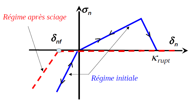
Figure 1.5-1: Illustration of the sawing procedure

This option is directly included in the parameters of the law of behavior. In practice, in order

to make the phenomenon close to physical reality, the sawn thickness is reduced by the initial joint opening before the operation. If the joint is in a strong initial opening, sawing will not affect it. On the other hand, if the joint is compressed, it will undergo complete sawing. Numerically, it will result in the change in the thickness parameter of the joint noted \({\delta }_{\mathrm{nf}}\), and, therefore, in a translation of the normal stress, such as:

(1.2)\[ {\ delta} _ {\ mathit {nf}} =\ mathit {nf}} =\ mathit {max} (\ mathrm {0,}} {\ delta}} _ {\ delta}}) - {\ delta}}) - {\ delta}} _ {\ delta} _ {\ mathit {saw}}\]

It is also considered that the joint in its final state is completely damaged by sawing. The latter, even if it is put into tension later, will therefore not develop any tensile strength. The procedure is explicit, combined with the elastic discharge for the overall structure that it generates, results in the rapid numerical convergence of the modeling. At most two Newton iterations are used, the first of which is used to update the thickness of the joints and the second is a linear discharge phase.

Note: Saw modeling is currently only available for basic laws JOINT_MECA_RUPT/FROT .Given the current numerical implementation, the phenomena of sawing and keying cannot be chained to the same joint.

1.6. Choice of parameters and application limits

The JOINT_MECA_RUPT/FROT laws of behavior are simple, robust, and dependent on few parameters. These laws do not make it possible to model the behavior in the break-friction transition phase. For the law of friction, which has a tensile strength that is not zero, joint failure is not implemented. Unlike these simplified behaviors, law JOINT_MECA_ENDO is a more complete law: it is capable of representing the evolution of the joint condition by combining the phenomena of rupture and friction.

The laws introduced have the significant advantage of being based on a theoretical formalism proven in the scientific literature. Some parameters are specific to the given law, others (such as hydro coupling) are universal in nature.

Parameters common to all laws

As all laws have an elastic phase and are compatible with hydromechanical coupling, some parameters are common to all laws.

Physical parameter	Aster name	Recommended value for concrete dams
Elastic behavior parameters
\({K}_{n}\) Normal stiffness	K_N	\({K}_{n}=3\cdot {10}^{12}\text{Pa/m}\)
\({K}_{t}\) Tangential stiffness	K_T	Flaw \({K}_{t}={K}_{n}\)
Hydromechanical coupling parameters
\({p}_{\mathrm{flu}}\) Imposed fluid pressure	PRES_FLUIDE	Defect \({p}_{\mathrm{flu}}=0\text{Pa}\) (absence of fluid)
\(\stackrel{ˉ}{\mu }\) Dynamic fluid viscosity	VISC_FLUIDE	\(\stackrel{ˉ}{\mu }={10}^{-3}\text{Pa}\cdot \text{s}\)
\(\rho\) Fluid density	RHO_FLUIDE	\(\rho \mathrm{=}1000{\text{kg/m}}^{3}\)
\({\epsilon }_{\mathrm{min}}\) Minimal joint opening	OUV_MIN	\({\epsilon }_{\mathrm{min}}={10}^{-8}\text{m}\)

Breaking behavior JOINT_MECA_RUPT

Physical parameter	Aster name	Recommended value for concrete dams
Common parameters of elastic behavior** + of the hydro coupling (see above)
\({\sigma }_{\mathrm{max}}\) Breakthrough threshold	SIGMA_MAX	\({\mathrm{\sigma }}_{\mathit{max}}=50\text{KPa}\)
\({P}_{\mathit{rupt}}\) Breakup penalty	PENA_RUPT	Flaw \({P}_{\mathit{rupt}}=1\)
\({P}_{\mathit{cont}}\) Contact penalty	PENA_CONTACT	Flaw \({P}_{\mathit{cont}}=1\)
\(\alpha\) Relative roughness	ALPHA	Flaw \(\alpha =1\)
\({\sigma }_{\mathit{nc}}\) Key pressure	PRES_CLAVAGE	Default \({\sigma }_{\mathit{nc}}=-1\text{Pa}\) (no keystroke)
\({\delta }_{\text{scie}}\) Saw size	SCIAGE	Defect \({\delta }_{\text{scie}}=0\text{m}\) (no sawing)

In the law JOINT_MECA_RUPTon has the possibility of penalizing the interpenetration of joint lips under additional compression. Parameter \({P}_{\mathit{cont}}\) is the ratio between compression stiffness and \({K}_{n}\) traction stiffness.

Friction behavior JOINT_MECA_FROT

Physical parameter	Aster name	Recommended value for concrete dams
Common parameters of elastic behavior** + of the hydro coupling (see above)
\(\mathrm{\mu }\) Coefficient of friction	MU	\(\mathrm{\mu }=1\)
\(c\) Membership	ADHESION	Flaw \(c=0\text{Pa}\)
\(\mathrm{{\rm K}}\) Isotropic work hardening	PENA_TANG	Flaw \(\mathrm{{\rm K}}=({K}_{n}+{K}_{t})\cdot {10}^{-6}\)
\({\mathrm{\sigma }}_{\mathit{nc}}\) Key pressure	PRES_CLAVAGE	Default \({\mathrm{\sigma }}_{\mathit{nc}}=-1\text{Pa}\) (no keystroke)
\({\mathrm{\delta }}_{\text{scie}}\) Saw size	SCIAGE	Defect \({\mathrm{\delta }}_{\text{scie}}=0\text{m}\) (no sawing)

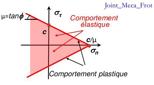
Figure 1.6-1: Elastic domain of law JOINT_MECA_FROT

Law JOINT_MECA_FROTest completely defined by its charge surface, as can be seen above. Isotropic work hardening \(\mathrm{{\rm K}}\) is introduced in order to regulate the mechanical response for force loads.

Figure 1.6-2: Movement generated by the kinematic hardening of the load surface (top) and the corresponding force-displacement response (bottom) for law JOINT_MECA_ENDO, for normal loading (left) for shear (right)

Coupling behavior: breakage and friction JOINT_MECA_ENDO

Physical parameter	Aster name	Recommended value for concrete dams
Common parameters of elastic behavior** + of the hydro coupling (see above)
\(\mathrm{\mu }\) Coefficient of friction	MU	\(\mathrm{\mu }=1\)
\({B}_{n}\) Normal movie work hardening	B_n	Unit \(\text{Pa/m}\)
\({B}_{t}\) Tangent movie work hardening.	B_t	Unit \(\text{Pa/m}\)
\({D}_{1}\) Breakup penalty	PENA_RUPT	Unit \(\text{Pa}\cdot \text{m}\)

The amplitudes of kinematic coupling \({B}_{n},{B}_{t}\) influence the tensile and shear peak values. The corresponding theoretical expressions were obtained in Ilaria Fontana’s thesis [Fontana2022]. We are listing them here without demonstration [2] _ . For the sake of consistency of the ratings with the thesis manuscript, the parameter for penalizing breakage is noted \({D}_{1}\). The apparent adhesion \(C\) representing the value of the peak shear is given by (eq. 2.43 of the thesis):

(1.3)\[ C=0.54\ cdot\ sqrt {2 {D} _ {1} _ {1} ({\ mathrm {\ mu}}} ^ {2} {B} _ {n} + {B} _ {t})}\]

The tensile strength noted \(T\) (same physical meaning as \({\mathrm{\sigma }}_{\mathit{max}}\) of the law JOINT_MECA_RUPT where \({R}_{t}\) JOINT_MECA_FROT) is given by (eq. 2.47 of the thesis):

\[\]

: label: eq-4

T=0.54cdotsqrt {2 {D} _ {1} {B} _ {n}}

The illustrates the physical meaning of parameters \(T\text{et}C\).

The values of the amplitudes of kinematic coupling \({B}_{n},{B}_{t}\) must respect the condition of absence of snap-back and of the simultaneous evolution of damage (proposal 2.6 of the thesis [3] _ ):

\[\]

: label: eq-5

begin {array} {c} 0<textcolor [rgb] {1,0,0} {1,0,0} {{B}} {{B}}le 1.31cdottext {min} ({K} _ {t} /2; {mathrm {mu}} /2; {mathrm {mu}}}}} ^ {1}}} ^ {2} {K} _ {n}} ^ {2} {K} _ {n})\ textcolor [rgb] {1,0,0}} {{B} _ {t}} /2; {mathrm {mu}}} /2; {mathrm {mu}}}} ^ {2} {K} _ {n})\ textcolor [rgb] {1,0,0}} {{B} _ {t} {mathrm {mu}} ^ {2} <textcolor [rgb] {0, .5,0} {{B} _ {n}}letext {min}left ((1.31cdot {K} _ {K} _ {2} _ {2}} <textcolor [rgb] {0, .5,0}} {{B}}}left ((1.31cdot {K}} _ {2}})/{mathrm {mu}} _ {2}} ^ {2}; 1.31 {K} _ {n}right)end {array}

Figure 1.6-3: Eligible domain for \({B}_{n},{B}_{t}\).

Two strategies for choosing parameters for the JOINT_MECA_FROT law

First strategy based on physical measurements

To have a non-empty set of possible value pairs constrained by eq, the following condition must be respected:

(1.4)\[ \ mathrm {\ mu} T\ le C\ le\ le\ sqrt {2}\ mathrm {\ mu} T\]

This last equation imposes the limits of choice for the apparent value of adhesion to the fixed tensile strength. Initially, the values of physical parameters \(T\text{et}C\) (values in units of stress) are chosen in order to best fit the load surface (obtained experimentally for example). The equations and make it possible to find the pair \(\overline{{B}_{n}}={B}_{n}{D}_{1}\) and \(\overline{{B}_{t}}={B}_{t}{D}_{1}\) and to set the ratio \({B}_{n}/{B}_{t}\) regardless of the choice of \({D}_{1}\). We then proceed to fix the values of the amplitudes of the kinematic coupling \({B}_{n},{B}_{t}\) on the basis of inequalities eq. By choosing \({D}_{1}\) which respects these inequalities. For very large values of \({D}_{1}\) the inequalities eq. Are automatically respected, because \(\underset{{D}_{1}\to \mathrm{\infty }}{\mathrm{lim}}{B}_{n,t}=0\). There is therefore a minimum value of \({D}_{1}\) that makes it possible to meet the condition of no snap-back. The closer you are to this value, the more robustness will be affected.

(1.5)\[ \begin{align}\begin{aligned} {D} _ {1}\ ge {D} _ {\ mathit {min}} =\ text {max}}} =\ text {max}\ left (\ frac {{T} ^ {2}}} {2}} {2}} {2}}\ frac {{D}} ^ {n}}}} {2}}\ right)\ cdot 0.76/ {0.54} _ {n}}}};\ frac {{C}}}} {n}}};\ frac {{C}}}}};\ frac {{C}} ^ {2}};\ frac {{C}} ^ {2}};\ frac {{C}} ^ {2}}\\ **Second strategy that prioritizes digital robustness**\end{aligned}\end{align} \]

We always rely on inequalities eq. By choosing pair \({B}_{n},{B}_{t}\) directly. \({B}_{t}\) can be set first, which establishes the \({B}_{n}\) variation limits. You should know that the greater the value of \({B}_{n}\) the closer we get to the behavior with the snap-back, which will make convergence more difficult. Once the \({B}_{n},{B}_{t}\) pair is chosen, the value of \({D}_{1}\) is adjusted in order to increase/reduce the size of the elastic zone according to the equations and. The values of \({D}_{1}\) are then of any kind belonging to the interval \((0;\mathrm{\infty })\).

[1]

Since this value is a hydraulic flow multiplier, its unit can be chosen so as to have the flows and mechanical stresses of the same order of magnitude, which simplifies error analysis.

[2]

We take \({m}_{1}=3;{m}_{2}=0.5\) which gives \({\mathrm{\alpha }}_{\mathit{max}}=0.0619\text{et}S({\mathrm{\alpha }}_{\mathit{max}})/\sqrt{-S\text{'}({\mathrm{\alpha }}_{\mathit{max}})}=0.542\)

[3]

for \({m}_{1}=3;{m}_{2}=0.5\to {\mathrm{\alpha }}_{\mathit{max}}=0.0619;\text{max}[R(\mathrm{\alpha })]=0.763={1.31}^{-1};S({\mathrm{\alpha }}_{\mathit{max}})/\sqrt{-S\text{'}({\mathrm{\alpha }}_{\mathit{max}})}=0.542\)