2. Theoretical formulation of JOINT_MECA_RUPT#

Law JOINT_MECA_RUPT accepts coupled hydromechanical modeling, but these two phenomena can be treated separately. First, we will describe the mechanical part of the law, which includes breakage, contact, locking procedure and imposed pressure. It is based on models XXX_JOINT (R3.06.09).

Note:The next two sections present the general theoretical concept. At first reading we can omit them and go directly to section § 2.3, which provides enough information to understand the numerical implementation of the law.

2.1. Cohesive law in mechanics#

The theoretical framework chosen to model the failure of concrete dam joints is based on cohesive models (R7.02.11,,), because in fragile failure, to avoid the problem of infinite stresses at the bottom of the crack, it is possible to introduce cohesive forces that impose a stress initiation criterion. The evanescent forces are then exerted between the particles on either side of the plane of separation of the crack during its opening (see Figure).

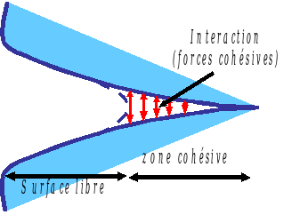
Figure 2.1-1: Diagram of a cohesive crack

From a physical point of view, it is considered that the opening of the crack costs an energy proportional to its length in 2D and to its surface in 3D. It’s called surface energy and it’s expressed using the energy density \(\Psi ={\int }_{\Gamma }\psi (\vec{\delta })d\Gamma\) [4] _ . The equilibrium displacement field \(\mathrm{u}\) is obtained by minimizing the sum of elastic energy \(\Phi\), surface energy, and the work of external forces \({W}^{\mathrm{ext.}}\). The solution is obtained using a variational approach to rupture. The state that achieves the minimum of total energy corresponds to a state of mechanical equilibrium:

(2.1)#\[ \ underset {\ mathrm {u}} {\ text {min}}}\ left (\ mathrm {\ Phi} (u) +\ mathrm {\ Psi} (\ vec {\ mathrm {\ delta}}} (u)) + {W} ^ {\ mathit {ext}}\ right)\]

The discontinuity surface is discretized in 2D or 3D by finite joint elements (see documentation R3.06.09). The displacement jump in element \(\vec{\delta }=({\delta }_{n},{\delta }_{\mathit{t1}},{\delta }_{\mathit{t2}})\) is a linear function of nodal displacements. The force [5] _ The coefficient of cohesion that is exerted on the lips of the crack is noted \(\vec{\sigma }\), it is defined by the derivative of the surface energy density with respect to the displacement jump. A relationship between \(\vec{\sigma }\) and the movement jump \(\vec{\delta }\) is called cohesive law. The most relevant material parameters, which describe the joint of a dam, are:

the two rigidities under normal stress \({K}_{n}\) and tangential \({K}_{t}\) stress, which characterize the surface and the materials used to fill the crack;
and the critical stress at break \({\mathrm{\sigma }}_{\mathit{max}}\)

In addition, three dimensionless numerical parameters are introduced: \({P}_{\mathit{rupt}}\), \({P}_{\mathit{cont}}\) and \(\mathrm{\alpha }\). The first controls the regularization of the softening slope during breakage, the second controls the penalization of contact and the third ensures a gradual resumption of tangential forces according to the normal opening. The latter can be associated with the relative size of the asperities of the surfaces in contact: \(\mathrm{\alpha }\in [\mathrm{0,2}]\).

In standard cohesive laws (R7.02.11) the surface energy depends on the displacement vector [6] _ and the constraints are defined as the first derivatives of energy:

(2.2)#\[ \begin{align}\begin{aligned} {\ mathrm {\ sigma}} _ {n} =\ frac {\ partial {\ partial {\ mathrm {\ psi}} _ {n} ({\ mathrm {\ delta}}} _ {n}})} {\ partial {\ mathrm {\ delta}} _ {n}}\\ \ textrm {and}\\ \ vec {{\ mathrm {\ sigma}} _ {t}}} =\ frac {\ partial {\ mathrm {\ psi}} _ {t} (\ vec {{\ mathrm {\ delta}}} _ {delta}}} _ {\ delta}}} _ {\ delta}} _ {\ delta}}} _ {\ delta}}} _ {\ delta}}} _ {\ delta}}} _ {\ delta}}} _ {\ delta}}} _ {\ delta}}\end{aligned}\end{align} \]

With energy:

(2.3)#\[ \ mathrm {\ Psi} (\ vec {\ mathrm {\ delta}}})\ equiv {\ int} _ {\ mathrm {\ Gamma}}\ mathrm {\ psi} ({\ mathrm {\ delta}}} ({\ mathrm {\ delta}}} ({\ delta}}) ({\ mathrm {\ delta}}) ({\ mathrm {\ delta}}) ({\ mathrm {\ delta}}} ({\ mathrm {\ delta}}} ({\ mathrm {\ delta}}} ({\ mathrm {\ delta}}}) ({\ mathrm {\ delta}}} ({\ mathrm {\ delta}}} ({\ mathrm\]

Unlike these standard cohesive laws, in this model, only the normal part of the law is derived from surface energy, while the tangential component of the law is given explicitly [7] _ .

In both cases, the irreversibility of the cracking is taken into account via a condition of increasing the maximum normal joint opening.

2.2. Surface energy for normal behavior#

The surface energy density \(\mathrm{\psi }\), at a given point in the crack, depends explicitly on the normal displacement jump between the lips of the crack \({\mathrm{\delta }}_{n}\). It also varies according to the condition of the joint, which is taken into account via an internal threshold variable \(\mathrm{\kappa }⩾0\), which manages the irreversibility of the cracking. The latter remembers the highest jump norm reached during the opening. Its law of evolution between two successive loading increments \(\text{-}\) and \(\text{+}\) is written as:

(2.4)#\[ {\ mathrm {\ kappa}}} ^ {\ text {+}}} =\ text {+}} =\ text {+}} =\ text {\ kappa}} ^ {\ text {-}}}, {\ mathrm {\ delta}}} _ {n}} ^ {\ text {-}}}, {\ mathrm {\ delta}}} _ {n} ^ {\ text {+}})\]

Depending on the opening value of the joint, we may find ourselves in one of these three situations:

The compressed joint is in the contact regime;
For a positive normal opening, if it exceeds the threshold, we speak of a dissipative regime (energy dissipation during cracking);
In the intermediate case, the joint is in a linear regime (linear discharge or recharge without energy dissipation).

The normal part of energy is written as:

(2.5)#\[\begin{split} {\ mathrm {\ psi}} _ {n} ({\ mathrm {\ delta}}} _ {n},\ mathrm {\ kappa}) =\ {\ begin {array} {ccc} {\ mathrm {\ psi}} {\ mathrm {\ psi}} {\ mathrm {\ psi}} {\ mathrm {\ psi}} {\ mathrm {\ psi}} {\ mathrm {\ psi}}} {\ mathrm {\ psi}} {\ mathrm {\ psi}}} {\ mathrm {\ psi}} {\ mathrm {\ psi}}} {\ mathrm {\ psi}}} {\ mathrm {\ psi}} {\ mathrm {\ psi}} {n}} {\ kappa})\ hfill &\ text {si} & {\ mathrm {\ delta}} _ {n} <0\\ {\ mathrm {\ psi}} _ {n} ^ {\ mathit {lin}}} {\ mathit {lin}}} & {\ lin}} ({\ mathrm {\ delta}}} _ {n},\ mathrm {\ kappa}} _ {n})\ hfill &\ text {si} {lin}}} ({\ mathit {lin}}}} ({\ mathrm {\ delta}}} _ {n})\ hfill &\ text {si} lin}}} ({\ mathit {lin}}}} ({\ mathrm {\ delta}}} _ {n})\ hfill {\ mathrm {\ delta}} _ {n} <\ mathrm {\ kappa} <\ mathrm {\ kappa}}\\ {\ mathrm {\ delta}} <\ mathrm {\ delta}} <\ mathrm {\ delta}} <\ mathrm {\ delta}}} ({\ mathrm {\ delta}}} ({\ mathrm {\ delta}}} ({\ mathrm {\ delta}}} ({\ mathrm {\ delta}}}) <\ mathrm {\ delta}}} ({\ mathrm {\ delta}}} ({\ mathrm {\ delta}}}} ({\ mathrm {\ delta}}} ({\ mathrm {\ delta}}} _ {n}\ kappa}\ end {array}\end{split}\]

And the tangential part:

(2.6)#\[\begin{split} {\ mathrm {\ psi}} _ {t} (\ vec {{\ mathrm {\ delta}}} _ {t}}) =\ {\ begin {array} {ccc} {\ mathrm {\ psi}} {\ mathrm {\ psi}}} _ {\ psi}}} _ {psi}}} _ {psi}}} _ {psi}} _ {psi}} _ {psi}}} _ {psi}} _ {psi}} _ {psi}} _ {psi}} _ {psi}} _ {psi}} _ {psi}} _ {psi}} _ {psi}}} _ {psi}} _ {psi}}} _ {psi}}} _ {psi}}} _ {psi}}} _ {psi}}} _ {psi}}} _ & {\ mathrm {\ delta}} _ {n} <0\\ {\ mathrm {\ psi}} _ {t} ^ {\ mathit {ouv}} (\ vec {{\ mathrm {\ delta}}} _ {delta}} _ {delta}} _ {\ mathrm {\ delta}}} (\ vec {\ mathrm {\ delta}}} (\ vec {\ mathrm {\ delta}}} _ {\ mathrm {\ delta}}} (\ vec {\ mathrm {\ delta}}} _ {\ mathrm {\ delta}}} (\ vec {\ mathrm {\ delta}}} _ {\ mathrm {\ delta}}} _ {\ mathrm {\ delta}}\end{split}\]

In summary, surface energy is written as follows:

(2.7)#\[ \ mathrm {\ psi} ({\ mathrm {\ delta}}} _ {n},\ mathrm {\ kappa}) =H ({\ mathrm {\ delta}} _ {n} -\ mathrm {\ kappa}}) {\ mathrm {\ kappa}}) {\ mathrm {\ kappa}) {\ mathrm {\ kappa}) {\ mathrm {\ kappa}) {\ mathrm {\ kappa}) {\ mathrm {\ kappa}) {\ mathrm {\ kappa}) {\ mathrm {\ kappa}) {\ mathrm {\ delta}}} _ {n})\ text {+} H ({\ mathrm {\ delta}}} _ {n})\ cdot H (\ mathrm {\ delta}} - {\ mathrm {\ delta}} _ {n}} _ {n}) {\ mathrm {\ delta}}) {\ mathrm {\ delta}} _ {n}) {\ mathrm {\ delta}} _ {n}) {\ mathrm {\ delta}} _ {n}) {\ mathrm {\ delta}} _ {n}) {\ mathrm {\ delta}} _ {n}) {\ mathrm {\ delta}} _ {n}) {\ mathrm {\ delta}} _ {n}) {\ mathrm {\ delta}} _},\ mathrm {\ kappa}) +H (- {\ mathrm {\ delta}} _ {n})\ cdot {\ mathrm {\ psi}} _ {n} ^ {\ mathit {con}} ^ {\ mathit {con}}} ({\ mathrm {\ delta}} _ {n})\]

Where \(H(x)\) is the Heaviside function (\(H(x)=0\text{si}x<\mathrm{0,}H(x)=1\text{si}x⩾0\)).

One of the particularities of law JOINT_MECA_RUPT is that, regardless of the regime, the behavior is always linear in terms of constraints. At the level of energies, we obtain quadratic functions, which are given next to one additive constant, which depends on the threshold.

The normal joint behavior is divided into three regimes: contact, linear and dissipative. The \({\psi }_{n}^{\mathit{con}}({\delta }_{n})=\frac{{P}_{\mathit{con}}{K}_{n}{\delta }_{n}^{2}}{2}\) function ensures the contact condition (no interpenetration of the crack lips) it is regularized in order to obtain better numerical convergence. By varying parameter \({P}_{\mathrm{con}}\), you can change the normal stiffness for the closed joint.

In linear regime, in the case where an existing crack evolves without dissipating energy, the corresponding energy density depends only on the normal stiffness parameter: \({\psi }_{n}^{\mathit{lin}}({\delta }_{n},\kappa )=\frac{{K}_{a}(\kappa ){\delta }_{n}^{2}}{2}\), where \({K}_{a}(\kappa )=({P}_{\mathit{rupt}}^{-1}+1){\sigma }_{\mathit{max}}/\kappa -{K}_{n}{P}_{\mathit{rupt}}^{-1}\) is a decreasing function of the rupture threshold \(\kappa\).

In the dissipative regime, in order to obtain linear softening, the corresponding energy density has a quadratic form as a function of the aperture:

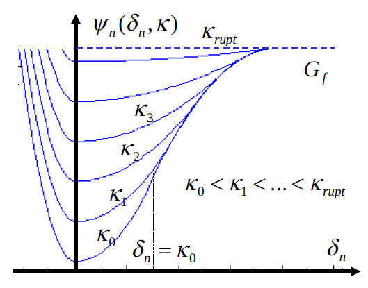
(2.8)#\[ {\ psi} _ {n} ^ {\ mathit {dis}}} ({\ delta} _ {n}) =\ {\ begin {array} {ccc} {\ sigma} _ {\ mathit {max}} (1+ {P}}} (1+ {P}} _ {P} _ {P} _ {P} _ {P} _ {n} {P} _ {n} {P} _ {P} _ {P} _ {P} _ {P} _ {P} _ {P} _ {P} _ {P} _ {P} _ {P} _ {P} _ {P} _ {P} _ {P} _ {P} _ {P} _ {P} _ {P} _ {P} _ {P} _ {P} _ {P} _ {P}} _ {\ mathit {rupt}} ^ {-1} {\ delta}} {\ delta} _ {n} ^ {2} /2&\ text {si} & {\ delta} _ {\ sigma} _ {\ sigma} _ {\ mathit {max}}} (1+ {P}} _ {\ mathit {rupt}})/{\ mathit {rupt}})/{\ mathit {rupt}})/{\ mathit {rupt}})/{\ mathit {rupt}})/{K} _ {\ sigma} _ {\ sigma} _ {\ sigma} _ {\ sigma} _ {\ sigma} _ {\ sigma} _ {\ sigma} _ {\ sigma} _ {\ sigma} _ {\ sigma} _ {\ sigma} _ {\ sigma} _ {\ sigma} _ {^ {2} {(1+ {P} _ {\ mathit {rupt}}})}}} ^ {2}/({\ mathrm {2P}}} _ {K} _ {n}) &\ text {si} {n}) &\ text {si}} & {\ mathit {rupt}}) &\ text {si} & {\ delta} & {\ delta} _ {\ mathit} _ {\ mathit {max}}} (1+ {P} _ {n}) &\ text {si} & {\ delta} & {\ delta} _ {\ mathit} {rupt}})/{K} _ {n}\ end {array}\]

Figure 2.2-1: Surface energy density as a function of the displacement jump for various values of the damage threshold \(\kappa\) The additive constant causes the elastic energies \({\psi }_{n}^{\mathit{lin}}\) and \({\psi }_{n}^{\mathit{con}}\) defined above to translate so that regardless of the state of damage to the joint, the same energy recovery rate is always obtained (Griffith constant \({G}_{f}\), see Figure and eq.). It only depends on the threshold and does not affect the expression of the constraints.

\({P}_{\mathrm{rupt}}\) is introduced in such a way that the more it increases, the greater the critical opening at breakage and, as a result, the more the dissipative energy of Griffith \({G}_{f}\) increases.

In summary: the normal behavior of the law JOINT_MECA_RUPT is driven by the evolution of the surface energy density, which is in the form of a potential sink. It has three main regimes: contact, linear elastic traction, damage/softening, whose corresponding profiles are approximated by quadratic opening functions. The joint starts to damage when the normal stress reaches the critical value \({\sigma }_{n}={\sigma }_{\mathit{max}}\). The more the joint is damaged the more the energy sink flattens see (Figure ). The damage parameter (the threshold) changes only in this last regime starting from its initial value for the healthy join \({\kappa }_{0}={\sigma }_{\mathit{max}}/{K}_{n}\) up to the ultimate value for the completely damaged join \({\kappa }_{\mathit{rupt}}={\sigma }_{\mathit{max}}(1+{P}_{\mathit{rupt}})/{K}_{n}\). \({P}_{\mathit{con}}\) is a constant defined by the user that changes the level of penalty in contact (see Figure ) . \({P}_{\mathrm{rupt}}\) changes the energy dissipated per unit area unit \({G}_{f}={\sigma }_{\mathrm{max}}^{2}(1+{P}_{\mathrm{rupt}})/({\mathrm{2K}}_{n})\)* is a constant defined by the user that changes the level of penalty in contact (see Figure ) .) .* changes the energy dissipated per unit area unit. In the end, we get the following expression for normal energy:

(2.9)#\[\begin{split} {\ psi} _ {n} (\ textcolor [rgb] {0,0.1} {0,0.1} {{\ delta}} _ {n}},\ kappa) =\ {\ begin {array} {\ ccc} {\ sigma} _ {\ mathit {max}} _ {\ mathit {max}}} {\ mathit {max}}}} (\ kappa - {\ kappa}} {\ sigma} _ {max}}} (1+ {P}}) _ {0}} (1+ {P}} _ {0}) /2+ {P} _ {\ mathit {con}} {K}} {K} _ {n}\ textcolor [rgb] {0,0.1} {{\ delta} _ {n} ^ {2}} /2&\ text {si} & {\ delta} & {\ delta} & {\ delta} & {\ delta}} _ {\ delta}} _ {\ delta} & {\ delta} & {\ delta}} _ {\ delta} _ {\ delta} _ {\ delta} _ {\ delta} _ {\ delta} _ {\ delta} _ {\ delta}} _ {\ delta} _ {\ delta} _ {\ delta} _ {\ delta} _ {\ delta} _ {\ delta}} _ {\ delta} _ {\ delta} _ {\ delta}} _ {\ delta} _ {\ delta -1}) (\ kappa - {\ kappa} _ {0}) /2+\ left [{\ sigma} _ {\ mathit {max}} (1+ {P} _ {\ mathit {rupt}}} ^ {-1}} ^ {-1})/\ kappa - {-1} -1}} ^ {-1}} ^ {rupt}} ^ {rupt}}} ^ {rupt}} ^ {rupt}}} ^ {rupt}}} ^ {rupt}} ^ {rupt}}} ^ {rupt}} ^ {rupt}}} ^ {rupt}} ^ {rupt}}} ^ {rupt}} ^ {rupt}}} ^ {rupt}} ^ {rupt}} ^ {rupt}}} ^ {rupt}} ^ {rupt}} ^ {rupt}} ^ {rupt}} ^ {rupt}} 0.1} {{\ delta} _ {n} ^ {2}} /2&\ text {si}} & 0{\ delta} _ {n} <\ kappa\\ {\ sigma} _ {\ mathit {max}} _ {\ mathit {max}}} (1+ {P}} _ {\ mathit {rupt}}} ^ {- 1}) (\ textcolor [rgb] {0,0.1} {0,0.1} {{\ delta} _ {n}}} - {\ kappa} _ {0} /2)\ text {-} {K} _ {n} {P} _ {\ P} _ {\ P} _ {P} _ {P} _ {P} _ {P} _ {P} _ {P} _ {P} _ {P} _ {P} _ {P} _ {P} _ {P} _ {P} _ {P} _ {P} _ {P} _ {P} _ {P} _ {P} _ {P} _ {P} _ {P} _ {P} _ {P} _ {P} _ {P} _ {P} _ {P} _ {P} _ {P} _ {P} _} &\ kappa {\ delta} _ {n} _ {n} < {\ kappa} < {\ kappa} _ {\ delta} _ {f} &\ text {si} & {\ delta} _ {\ delta} _ {n} _ {n} {\ kappa}} _ {\ mathit {rupt}} {f} &\ text {si} & {\ delta}} _ {\ delta} _ {\ delta} _ {\ delta} _ {n} {\ kappa}} _ {\ kappa} _ {\ mathit {rupt}}\ end {array}\end{split}\]

This function is continuous and differentiable, which ensures the continuity of the constraints.

2.3. Constraint vector#

The stress vector in the element is denoted \(\vec{\sigma }=({\sigma }_{n},\vec{{\sigma }_{t}})\) [8] _ , it can be separated into several regimes. For the normal part, the stress vector is equal to the sum of the derivatives of the surface energy density and the penalization energy density in contact with respect to the jump.

(2.10)#\[ {\ sigma} _ {n} =H ({\ delta} _ {n} _ {n} -\ kappa) {\ sigma} _ {n} ^ {\ mathit {dis}} +H (\ kappa - {\ delta} _ {n} _ {n}) H ({\ delta} _ {n}) H ({\ delta} _ {n}) H (- {\ delta} _ {n}) H ({\ delta} _ {n}) H ({\ delta} _ {n}) H ({\ delta} _ {n}) H ({\ delta} _ {n}) H ({\ delta} _ {n}) H ({\ delta} _ {n}) H ({\ delta} _ {n}) H ({\ delta} _ {n}) H (\ delta n}) {\ sigma} _ {n} ^ {\ mathit {con}}\]

It is therefore sufficient to derive the expressions given in the previous section (§ 2.2) to obtain the normal component of the constraints [9] _ . The tangential part \({\overrightarrow{\sigma }}_{t}^{\mathrm{fer}}=f({K}_{t},\overrightarrow{{\delta }_{t}})\) is written as:

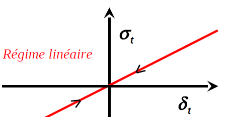
(2.11)#\[ {\ vec {\ mathrm {\ sigma}}}} _ {t}} = H ({\ mathrm {\ delta}} _ {n}) {\ vec {\ mathrm {\ sigma}}}} _ {t}} ^ {\ t} ^ {\ mathit {ouv}} ^ {\ mathit {ouv}}} +H (- {\ mathrm {\ delta}} _ {n}) {\ vec {\ mathrm {\ sigma}}}} _ {t} ^ {\ t} ^ {\ mathit {ouv}} ^ {\ mathit {ouv}} +H (- {\ mathrm {\ delta}} _ {n}) {\ vec {\ mathrm {\ sigma}}}} _ {t}} ^ {\ t}}} _ {t} ^ {\ mathit {fer}}\]

This is a function of the tangential opening, it involves the tangential stiffness for the closed joint. Depending on the profile of the interface, the tangential behavior for the open joint can be varied \({\vec{{\sigma }_{t}}}^{\mathit{ouv}}={\vec{{\sigma }_{t}}}^{\mathit{fer}}\) for jagged surfaces (as for example in the Figure on the right), or \({\overrightarrow{{\sigma }_{t}}}^{\mathrm{ouv}}\equiv 0\) for very smooth surfaces (Figure on the left).

2.3.1. Normal stresses#

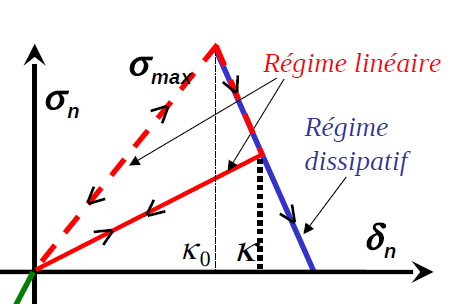
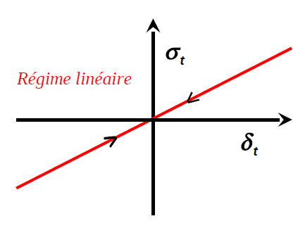
Consider the expression normal constraint:

(2.12)#\[ {\ sigma} _ {n} ({\ delta} _ {n} _ {n},\ kappa) =\ {\ begin {array} {ccc} {P} _ {\ mathit {con}} {K} _ {n} {\ delta} _ {\ delta} _ {\ delta} _ {n} _ {\ mathit {max} _ {\ mathit {max}} (1+ {P} _ {\ mathit {rupt}}} ^ {-1}})/\ kappa - {K} _ {n} {P} _ {\ mathit {rupt}} ^ {-1}\ right] {\ right] {\ delta} {\ delta}} _ {\ delta} _ {\ sigma} _ {\ delta} _ {\ mathit {max} _ {\ mathit {max}} (1+ {P} _ {\ mathit {rupt}}} ^ {-1}})\ text {-} {-1})\ text {-} {K} _ {\ mathit {rupt}}} ^ {-1} {\ delta} _ {\ delta} _ {\ delta} _ {\ delta} _ {\ mathit {\ delta} _ {\ mathit {rupt}} _ {\ delta} _ {\ delta} _ {\ delta} _ {\ delta} _ {\ delta} _ {\ delta} _ {\ delta} _ {\ delta} _ {\ delta} _ {\ delta} _ {\ delta} _ {\ delta} _ {\ delta} _ {\ delta} _ {\ delta} _ {\ delta} _ {\ delta} _ {\ delta} _ {\ delta} _ {\ delta}\ text {si} & {\ delta} _ {n} {n} {\ kappa} _ {\ mathit {rupt}}\ end {array}\]

The evolution of this stress in the traction zone as a function of the jump is shown in FIG. The arrows represent the possible direction of evolution of the constraint depending on whether the opening process is reversible (linear regime) or not (dissipative regime). Upon initiation, the joint behaves first in a linear elastic manner, then as soon as the normal stress reaches the critical value \({\sigma }_{n}={\sigma }_{\mathrm{max}}\), it has a softening behavior: it gradually loses its stiffness, which gives the regime linear but not elastic, it is characterized by a slope of softening the break \(-{K}_{n}/{P}_{\mathrm{rupt}}\). The elastic stiffness for the healthy joint defines the initial value of damage threshold \({\kappa }_{0}={\sigma }_{\mathrm{max}}/{K}_{n}\). The breaking point is given by \({\kappa }_{\mathrm{rupt}}={\sigma }_{\mathrm{max}}(1+{P}_{\mathrm{rupt}})/{K}_{n}\). The more important \({P}_{\mathit{rupt}}\) is, the more the dissipation energy increases \({G}_{f}={\sigma }_{\mathrm{max}}^{2}(1+{P}_{\mathrm{rupt}})/({\mathrm{2K}}_{n})\).

Figure 2.3-1: Dependence of stresses as a function of opening

2.3.2. Constraint to penalize contact#

The value of the penalty slope in contact is given by the following relationship:

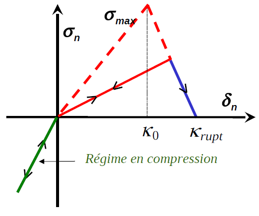
(2.13)#\[ \begin{align}\begin{aligned} {\ sigma} _ {n} ({\ delta} _ {n}) = {P} _ {\ mathit {con}} {K} _ {n} {n} {\ delta} _ {n}\\ \ textrm {if}\\ {\ delta} _ {n} <0\end{aligned}\end{align} \]

Figure 2.3-2: Normal cohesive stress as a function of the normal jump for the partially damaged joint

The numerical parameter PENA_CONTACT, given by the user, makes it possible to play on the slope of contact penalties (see Figure). By default, it is set to \(1\), which corresponds to the case where the contact slope is identical to that of the opening stiffness. If you choose a value greater than \(1\), you increase the penalty. This makes it possible to model, for example, the resumption of forces by concrete that is partially damaged in tension. For a value less than \(1\), the penalty is reduced, which makes it possible to simulate concrete that is partially damaged under compression.

2.3.3. Tangential stress#

For barrier joints with small openings, it is observed that regardless of the normal loading regime, the tangential stress always varies linearly, the tangential stiffness is a function of the normal opening. In the extreme case of a perfectly smooth contact surface, the tangential stiffness drops sharply to zero at the positive normal opening. As a result, the surface energy of the law is no longer continuous, which in principle generates a peak in the normal stress (delta function \(\textcolor[rgb]{1,0,0}{\delta }(x)\)) at the opening. For this reason, in the current version of the law, we renounce the need to maintain the complete energy formalism. The tangential law is then postulated empirically in linear form with the tangential stiffness dependent on the normal opening:

\[\]

: label: eq-21

vec {{mathrm {sigma}} _ {t}}} ({mathrm {delta}}} _ {t}, {mathrm {delta}} _ {n}) ={begin {array} {array} {{array} {{array} {{array} {{array} {{array} {{array} {{array} {ccc}} {K} {K}} _ {t}} - {vec {K}} _ {t}} - {vec {mathrm {delta}}} _ {mathit {shift}}}) &text {si}} & {mathrm {delta}} _ {n} <0\ (1- {mathrm {delta}}} _ {mathrm {delta}}} _ {mathrm {delta}}} _ {mathit {rupt}} <0(1- {mathrm {delta}}} _ {mathrm {delta}}} _ {mathrm {delta}}} _ {mathrm {tan}}}) {K} _ {t}cdot (vec {{mathrm {delta}}} _ {delta}}} - {vec {mathrm {delta}}} _ {mathit {shift}}}) &text {si}} & 0{mathrm {delta}} _ {mathrm {kappa}}} _ {mathit {shift}}) &text {si} & 0{mathrm {delta}}} _ {mathit {shift}}) &text {si} & 0{mathrm {delta}}} _ {mathit {shift}}) &text {si} & 0{mathrm {delta}}} _ {mathit {shift}}})}} ^ {mathrm {tan}}\ 0&0&text {si}} & {mathrm {delta}} _ {n} {mathrm {kappa}}} _ {mathit {rupt}}} _ {mathit {rupt}}} _ {mathit {rupt}}} _ {mathit {rupt}}} _ {mathit {rupt}}} _ {mathit {rupt}}}} _ {mathit {rupt}}} _ {mathit {rupt}}}} _ {mathit {rupt}}}

The story variable \(\vec{{\mathrm{\delta }}_{\mathit{shift}}}\) represents the shift from the balance point in tangential sliding to the open joint: \(\vec{{\mathrm{\delta }}_{\mathit{shift}}}\) is equal to the last value of \(\vec{{\mathrm{\delta }}_{t}}\) for which the joint was opened \({\mathrm{\delta }}_{n}\ge {\mathrm{\kappa }}_{\mathit{rupt}}^{\mathrm{tan}}\). We are introducing the tangential break threshold \({\mathrm{\kappa }}_{\mathit{rupt}}^{\mathrm{tan}}={\mathrm{\kappa }}_{\mathit{rupt}}\mathrm{tan}(\mathrm{\alpha }\mathrm{\pi }/4)\), whose value can be changed by the user with \(\alpha \in [\mathrm{0,2}]\) and the ALPHA keyword. For a zero value the tangential slope changes abruptly at the opening, for the value \(\alpha =2\) the tangential stiffness does not change. For the sake of compatibility with the laws of behavior developed in the Gefdyn code, we do not correct the normal component of the stresses in the transition phase, this is always given by (), which gives a non-symmetric tangent matrix and therefore the regime of uncontrolled dissipation. The evolution of the tangential stress is divided into three regimes: elastic joint under compression; elastic joint partially open with reduced stiffness; joint completely broken (see equation () and Figure.)

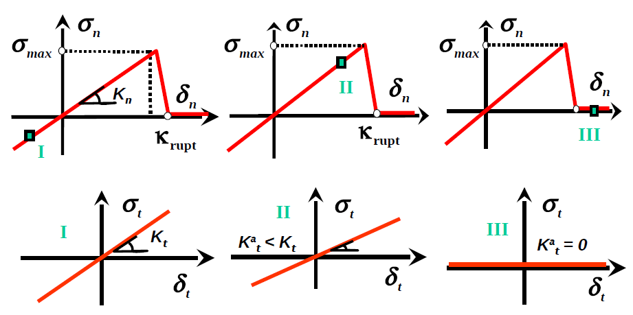
Figure 2.3-3: Illustration of the coupling between shear and normal joint opening: I in the compression regime; II in the partial opening regime; III in the full opening regime. We note \({K}_{t}^{a}\equiv (1-{\delta }_{n}/{\kappa }_{\mathrm{rupt}}^{\mathrm{tan}}){K}_{t}\)

2.4. Tangent operator#

As the behavior in each of the regimes is linear, the calculation of the tangent matrix is easy:

(2.14)#\[\begin{split} \ frac {\ partial {\ sigma} _ {n} ({\ delta} _ {n})} {\ partial {\ delta} _ {n}} =\ {\ begin {array} {ccc} {P} {P} _ {\ mathit {con}} _ {con}}} {K}} {K} _ {n} &\ text {\ delta} _ {n} _ {mathit {con}}} {\ sigma} _ {mathit {con}}} {K}} {K} _ {n} &\ text {\ delta} _ {n} _ {mathit {con}}} {it {max}} (1+ {P} _ {\ mathit {rupt}}} ^ {-1})/\ kappa - {K} _ {n} {P} _ {\ mathit {rupt}} ^ {-1}} ^ {-1} &\ text {-1} &\ text {1} &\ text {si} & 0{\ mathit {rupt}} & 0{\ delta} _ {\ delta} _ {n} {P} _ {P} _ {\ mathit {-1}} &\ text {si} & 0{\ delta} _ {\ delta} _ {n} {P} _ {P} _ {\ mathit {-1}} &\ text {si} & 0{\ delta} _ {\ delta} _ {rupt}} ^ {-1} &\ text {si} &\ kappa {\ delta} _ {n} < {\ kappa} _ {\ mathit {rupt}}\\ 0&\ text {si} & {\ delta} & {\ delta} & {\ delta} _ {n} {\ delta} _ {n} {\ delta} _ {\ mathit {rupt}}\ end {array}}\end{split}\]

(2.15)#\[ \begin{align}\begin{aligned} \ frac {\ partial {\ sigma} _ {n} _ {n} ({\ delta} _ {n})} {\ partial {\ delta} _ {t}} =0\\\begin{split} \ frac {\ partial\ vec {{\ sigma} _ {t}}} (\ vec {{\ delta} _ {t}}, {\ delta} _ {n})} {\ partial\ vec {{\ delta} _ {\ delta} _ {t}} _ {t}}} =\ {\ begin {array}}}} =\ {\ begin {array} {t}} _ {t}\ mathit {id} & {\ delta} _ {n} <0\\ (1- {\ delta} _ {n}} _ {n}/{n}/{k} _ {\ mathit {rupt}} ^ {\ mathrm {tan}}) {K} _ {t}\ mathit {Id} &\ text {Id} &\ text {id} &\ text {si}/{si} & 0{\ delta} _ {n} < {\ kappa}} _ {\ mathit {rupt}}} ^ {\ mathrm {Id}} &\ text {si} & 0{\ delta} _ {n} < {\ kappa}} _ {\ mathit {rupt}}} ^ {\ mathrm {Id}} &\ text {si} & 0{\ delta} _ {n} _ {}}\\ 0&\ text {si} & {\ delta} & {\ delta} _ {n} {\ kappa} _ {\ mathit {rupt}}} ^ {\ mathrm {tan}}}\ end {array}}\end{split}\end{aligned}\end{align} \]

(2.19)#\[\begin{split} \ frac {\ partial\ vec {{\ sigma} _ {t}}} (\ vec {{\ delta} _ {t}}, {\ delta} _ {n})} {\ partial\ vec {{\ delta} _ {\ delta} _ {t}} _ {t}}} =\ {\ begin {array}}}} =\ {\ begin {array} {t}} _ {t}\ mathit {id} & {\ delta} _ {n} <0\\ (1- {\ delta} _ {n}} _ {n}/{n}/{k} _ {\ mathit {rupt}} ^ {\ mathrm {tan}}) {K} _ {t}\ mathit {Id} &\ text {Id} &\ text {id} &\ text {si}/{si} & 0{\ delta} _ {n} < {\ kappa}} _ {\ mathit {rupt}}} ^ {\ mathrm {Id}} &\ text {si} & 0{\ delta} _ {n} < {\ kappa}} _ {\ mathit {rupt}}} ^ {\ mathrm {Id}} &\ text {si} & 0{\ delta} _ {n} _ {}}\\ 0&\ text {si} & {\ delta} & {\ delta} _ {n} {\ kappa} _ {\ mathit {rupt}}} ^ {\ mathrm {tan}}}\ end {array}}\end{split}\]

(2.17)#\[\begin{split} \ frac {\ partial\ vec {{\ mathrm {\ sigma}} _ {\ sigma}} _ {\ sigma}} _ {\ delta}}, {\ mathrm {\ delta}} _ {n}} _ {n}})} {\ partial {\ mathrm {\ sigma}}} _ {\ delta}}} =\ {\ begin {array} {\ delta}}}}, {\ mathrm {\ delta}}} _ {\ delta}}}, {\ mathrm {\ delta}}} _ {\ delta}}}, {\ mathrm {\ delta}}} _ {\ delta}}}, {\ mathrm {\ delta}}} _ {\ delta}}}, {\ mathrm {\ delta}}} _ {\ delta}}} if} & {\ mathrm {\ delta}}} _ {n} <0\\ - {K} _ {t} (\ vec {{\ mathrm {\ delta}}} _ {t}} - {\ vec {\ mathrm {\ delta}}} _ {\ mathrm {delta}}}} _ {\ mathit {delta}}} _ {\ mathit {rupt}}} - {\ vec {\ mathrm {delta}}} - {\ vec {\ mathrm {\ delta}}} - {\ mathrm {delta}}}} - {\ vec {\ mathrm {\ delta}}}} _ {\ mathrm {delta}}}} _ {\ mathrm {delta}}}} _ {\ mathrm {\ delta}}}}} &\ text {si} & 0{\ mathrm {\ delta}}} _ {n} < {\ mathrm {\ kappa}} _ {\ mathit {rupt}} ^ {\ mathrm {tan}}}\\ 0&\ mathrm {\ delta}}} _ {\ mathrm {\ delta}} _ {\ mathrm {\ kappa}}} _ {mathit {\ kappa}} ^ {\ mathrm {\ kappa}}} ^ {\ mathrm {\ tan}}}}\\ 0&\ text {\ delta}} _ {mathit {\ kappa}} ^ {\ mathrm {tan}}}} ^ {\ mathrm {tan}}}}\\ 0&\ text {\ delta}} _ {mathit it {rupt}} ^ {\ mathrm {tan}}\ end {array}\end{split}\]

Note that the tangent matrix is not symmetric. This results from the non-repercussion on the normal stresses of the regularization of the evolution of the tangential stress at the opening of the joint (singular terms are not taken into account).

2.5. Digital keyboard implementation#

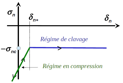
Cleavage corresponds physically to a procedure for injecting concrete grout under pressure between the pads of the dam; it is characterized by a simple parameter: the local pressure of injected grout \({\sigma }_{\mathit{nc}}⩾0\). To set up the key, the user must define a key pressure function, keyword PRES_CLAVAGE, which depends on both space (typing in different places at different pressures) and time (several successive keystrokes). Places where the key pressure is negative are not keyed.

The procedure is modelled by modifying the thickness of the joints concerned. If the joint is initially strongly compressed, the claving does not influence it. On the other hand, if the joint is open or not sufficiently compressed (i.e. if \({\sigma }_{n}>-{\sigma }_{\mathrm{nc}}\)), the locking will result in a change in the total thickness parameter of the joint noted \({\delta }_{\mathit{nf}}^{\text{+}}={\delta }_{\mathit{nf}}^{\text{-}}+{\delta }_{n}^{\text{+}}+{\sigma }_{\mathit{nc}}/({P}_{\mathit{con}}{K}_{n})\).

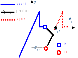
Cleaving then preserves the normal opening of each joint while translating the law of behavior along the abscissa axis. The new local equilibrium position has a normal stress equal to the pressure of injected concrete \({\sigma }_{n}=-{\sigma }_{\mathrm{nc}}\). This procedure is applied locally. Although each joint subjected to claving is found in the linear compression regime, the selection itself of the joints to be keyed is « non-linear ». As a result, the overall procedure also becomes non-linear and it is not enough to just modify the normal stresses of the keyed joints to obtain mechanical balance again after claving. Consequently, a mechanical balance calculation is carried out after this « local » claving to return the system to its state of equilibrium. If the clearance of the key joint is changed, the thickness of the joints is updated and so on as long as there are the points where \({\sigma }_{n}>-{\sigma }_{\mathrm{nc}}\) exist. The joints in question close and are gradually compressed while following the normal behavior curve. This procedure is only done once during the digital dam « construction » phase. An illustration is shown in the figure above. The « in » and « out » points correspond respectively to the values of the constraint before and after the key.

The normal behavior of the joint after claving can be changed. Thus, the tensile strength can be restored either partially or completely (this is the case in the figure) depending on the damage to the joints before the claving procedure. In the procedure as developed we made the choice not to restore the tensile strength, it maintains its current value.

Figure 2.5-1:. The evolution of normal stress during claving: joint partially damaged on the left and completely damaged on the right

In order to identify the tangent matrix for claving, it is useful to represent this procedure as a temporary modification of the initial law of behavior by an incremental law. For the tangential regime, the claving procedure does not require any modification: the associated stress always depends linearly on the tangential displacement and the loading slope varies according to the joint opening. Normal coupling deserves to be analyzed in more detail. Suppose we are in a given loading state \({\delta }_{n\text{+}}\) and we try to find the stress state that is infinitesimally close. First, let’s look at the case where \({\delta }_{n}\) is decreasing. Since the joint thickness was already updated at the previous Newton iteration, the joint falls into the compression domain and the activation of the key plays no role at this stage. We therefore find the compression slope of the initial law. On the other hand, if the joint is loaded with tension, the claving procedure is activated and the joint thickness is adapted in such a way as to make the normal stress ceiling by the locking pressure. In fact, the behavior becomes bilinear with a compression slope of the initial compression law and the slope in the traction zone, which is completely cancelled out (see Figure).

Figure 2.5-2:. Modification of the law of behavior during the claving phase

As the behavior in each of the regimes remains linear, calculating the tangent matrix is always easy:

(2.18)#\[ \begin{align}\begin{aligned}\begin{split} \ frac {\ partial {\ sigma} _ {n} ({\ delta} _ {n})} {\ partial {\ delta} _ {n}} =\ {\ begin {array} {ccc} {P} {P} _ {\ mathit {con}} _ {con}}} {K}} {K}} _ {n} &\ text {\ delta} _ {n} _ {n} _ {n} < {\ delta} _ {n} _ {n} _ {\ delta} _ {P} _ {P} _ {P} _ {P} _ {P} _ {\ mathit}}} {\ mathit}}} {n} f}}\\ 0&\ text {si} & {\ delta} & {\ delta} _ {\ delta} _ {\ mathit {nf}}}\ end {array}}\end{split}\\\begin{split} \ frac {\ partial\ vec {{\ sigma} _ {t}}} (\ vec {{\ delta}} _ {t}}, {\ delta} _ {n})} {\ partial\ vec {{\ delta} _ {\ delta} _ {t}} _ {\ delta} _ {\ delta} _ {\ delta} & {\ delta} _ {n} < {\ delta} _ {\ mathit {nf}}}\\ (1- {\ delta} _ {n}/{k} _ {\ mathit {rupt}}} ^ {\ mathrm {tan}}}) {\ mathrm {tan}}}) {K}}) {K} _ {t} {i} {I} {I} _ {d} & {\ delta} _ {\ mathit {nf}} {tan}}) {K}} {\ mathrm {tan}}}) {K}} {\ mathrm {tan}}) {K}}) {K}} {delta}}) {K}} {\ mathit {tan}}}) {K}} {delta}}} _ {n} < {\ kappa} _ {\ mathit {rupt}}} ^ {\ mathrm {tan}}\\ 0&\ text {si} & {\ delta} _ {n} {\ kappa} _ {\ kappa} _ {\ mathit {rupt}} _ {\ mathit {rupt}}} ^ {\ mathrm {tan}}}\ end {array}}\ end {array}\end{split}\end{aligned}\end{align} \]

(2.19)#\[\]

\[\]

: label: eq-27

frac {partial {sigma} _ {n} _ {n} ({delta} _ {n})} {partial {delta} _ {t}} =0

(2.20)#\[\begin{split} \ frac {\ partial\ vec {{\ sigma} _ {t}}} (\ vec {{\ delta}} _ {t}}, {\ delta} _ {n})} {\ partial\ vec {{\ delta} _ {\ delta} _ {t}} _ {\ delta} _ {\ delta} _ {\ delta} & {\ delta} _ {n} < {\ delta} _ {\ mathit {nf}}}\\ (1- {\ delta} _ {n}/{k} _ {\ mathit {rupt}}} ^ {\ mathrm {tan}}}) {\ mathrm {tan}}}) {K}}) {K} _ {t} {i} {I} {I} _ {d} & {\ delta} _ {\ mathit {nf}} {tan}}) {K}} {\ mathrm {tan}}}) {K}} {\ mathrm {tan}}) {K}}) {K}} {delta}}) {K}} {\ mathit {tan}}}) {K}} {delta}}} _ {n} < {\ kappa} _ {\ mathit {rupt}}} ^ {\ mathrm {tan}}\\ 0&\ text {si} & {\ delta} _ {n} {\ kappa} _ {\ kappa} _ {\ mathit {rupt}} _ {\ mathit {rupt}}} ^ {\ mathrm {tan}}}\ end {array}}\ end {array}\end{split}\]

(2.21)#\[\begin{split} \ frac {\ partial\ vec {{\ mathrm {\ sigma}} _ {\ sigma}} _ {\ sigma}} _ {\ delta}}, {\ mathrm {\ delta}} _ {n}} _ {n}})} {\ partial {\ mathrm {\ sigma}}} _ {\ delta}}} =\ {\ begin {array} {\ delta}}}}, {\ mathrm {\ delta}}} _ {\ delta}}}, {\ mathrm {\ delta}}} _ {\ delta}}}, {\ mathrm {\ delta}}} _ {\ delta}}}, {\ mathrm {\ delta}}} _ {\ delta}}}, {\ mathrm {\ delta}}} _ {\ delta}}} if} & {\ mathrm {\ delta}} _ {n}} _ {n} < {\ mathrm {\ delta}} _ {\ mathit {nf}}\\ - {K} _ {t} (\ vec {{\ mathrm {\ delta}}} _ {\ mathrm {\ delta}}} _ {\ mathit {shift}}} (\ vec {\ mathrm {\ delta}}})/{k})/{k} _ {\ mathit {rupt}} ^ {\ mathrm {\ delta}}} ^ {\ mathrm {\ delta}} _ {\ mathit {nf}} {\ mathrm {\ delta}}} ^ {\ mathrm {\ delta}}} _ {\ mathrm {\ delta}}} _ {\ mathrm {\ delta}}} _ {\ mathrm {\ delta}} _ {\ mathrm {\ delta}} _ {\ mathrm {\ delta}} _ {\ mathrm {\ delta}} _ {\ mathrm {\ delta}} _ {\ mathrm {\ delta}} _ {\ mathrm {\ delta}} _ {\ mathrm {\ delta}}} _ {\ mathrm {\ delta}} 0&\ text {si} & {\ mathrm {\ delta}}} _ {n} {\ mathrm {\ kappa}} _ {\ mathit {rupt}}} ^ {\ mathrm {tan}}}\ end {array}} ^ {\ mathrm {tan}}\end{split}\]

2.6. Internal variables#

Law JOINT_MECA_RUPT has eighteen internal variables. From the point of view of the law of behavior, only the first and the tenth are*stricto sensu* internal variables. The others provide information on the hydromechanical state of the joint at a given moment.

\(V1\)	Threshold \(\mathrm{\kappa }\) in jumping (highest norm reached).
\(V2\)	Dissipation indicator \(=0\) if linear regime, \(=1\) if dissipative regime.
\(V3\)	Normal damage indicator \(=0\) healthy, \(=1\) damaged, \(=2\) broken
\(V4\)	Percentage of normal damage (in the softening zone) \(V4\in [\mathrm{0,1}]\)
\(V5\)	Tangential damage indicator \(=0\) healthy, \(=1\) damaged, \(=2\) broken
\(V6\)	Tangential damage percentage \(V6\in [\mathrm{0,1}]\)
\(V7\)	Normal jump \({\mathrm{\delta }}_{n}\).
\(V8\) \(V9\)	Tangential jumps, respectively \({\mathrm{\delta }}_{t1}\) and \({\mathrm{\delta }}_{t2}\) (\(V9\) null in 2D).
\(V10\)	Thickness \({\mathrm{\delta }}_{\mathit{nf}}\) of the keyed joint.
\(V11\)	Normal mechanical stress \({\mathrm{\sigma }}_{n}\) (without fluid pressure)
\(V12\) \(V13\) \(V14\)	Components of the pressure gradient in the global coordinate system (only for modelsxxx_ JOINT_HYME). \({\partial }_{x}p\), \({\partial }_{y}p\), and \({\partial }_{z}p\) respectively.
\(V15\) \(V16\) \(V17\)	Hydraulic flow components in the global coordinate system (only for xxx_ JOINT_HYME models). \({w}_{x}\), \({w}_{y}\), and \({w}_{z}\) respectively.
\(V18\)	User imposed fluid pressure \(p\) (PRES_FLUIDE) in the case of models xxx_ JOINTou fluid pressure interpolated from that calculated at the middle nodes of the joint elements (degree of freedom of the problem) for the models: xxx_ JOINT_HYME.
\(V19\) \(V20\)	Two components of the tangential drag vector \(\vec{{\mathrm{\delta }}_{\mathit{shift}}}\)