4. Theoretical formulation of JOINT_MECA_ENDO#

One of the key points in the accurate description of interfaces between rocks is the identification of their elastic domain (also called load surface or the criterion). Because of their softening nature, not only rock contacts but also any kind of analogous interface involving similar materials such as concrete, clay or soil can generally be classified according to their resistance to various loads in mixed mode. This approach is closely linked to basic safety rules in industrial applications, where it is accepted as a first approximation that geomaterials could present an unstable failure once the critical load has been reached.

Throughout the last century, specific test machines and corresponding measurement protocols have been set up in order to harmonize and standardize the experimental characterization of the fragile interfaces mentioned above. To name but a few, simple tensile testing or fixed compression shear are both well-documented experiments that are performed in practice to catalog the strength of materials by identifying only a few points on their multidimensional elastic surface. This vision reduced « to a single point » of the resistance of materials has been increasingly scrutinized lately, and multiple developments have been adopted. For example, constant improvements in finite element software allow for new types of modeling, with loads that go beyond the elastic domain to explore more subtle post-peak behavior. While the complexity of post-peak description could be achieved through various theoretical formalisms, most of them still rely on the initial definition of the load surface, and the question of this form of elastic domain remains the cornerstone of any nonlinear model identification. Even though considerable progress has been made over the last few decades, this precise identification of the load surface remains a fairly difficult task today.

A common characteristic of geomaterials is their high resistance to compression loads. In current industrial applications, it is precisely this property of higher compressive strength that is exploited in order to increase the overall robustness of the structure. As the interfaces considered are composed of geomaterials, it is natural to assume a similarity between the corresponding load surfaces. For geomaterials, depending on their physical origin, a wide variety of criteria defining the elastic domain are used in order to model their mechanical behavior. The simplest surface, admitting infinite resistance in hydrostatic compression, is that in the shape of a linear cone. It was first introduced over a century ago [Mohr1900] as the combination of the Coulomb friction hypothesis [Coulomb1776] with the Galileo-Rankine voltage cutoff principle. The initial description of the principal stress, commonly referred to as the Mohr-Coulomb form, was then generalized in the work of Drucker and Prager to a smoother deviator-trace relationship [Drucker1952]. The direct relationship between shear and compression loads, which is the main signature of these linear criteria, has allowed the development of various constitutive relationships based on the same simplified dependence [Marigo2019]. At this stage, we note that the linear conical surface is currently commonly used to date for the modeling of geomaterials.

With many major infrastructure projects in progress, more complex criteria emerged as new experimental data became available. For wider load ranges, the compression shear dependence seemed to deviate from the linear curve. In 1980 Evert Hoek and Edwin T. Brown [Hoek1980] proposed a new particular form of criterion in a quadratic form. It reproduces the Mohr-Coulomb type singularity for low tensile loading while simultaneously taking into account the reduction in shear strength for high compression. This purely empirical criterion has been widely used in the design of underground excavations [Hoek1982]. More recent work on rock joints seems to show the same change in the load surface.

Law JOINT_MECA_ENDO attempts to partially capture this phenomenon, starting from the linear elastic load surface, the latter evolves thanks to kinematic work hardening, the tensile strength is captured by the damaging coupling of the strain hardening amplitude. The apparent shape of the load surface is no longer linear and as a result it approaches the load surfaces of the real joints. We also have the advantage of being able to represent the cohesive zone model and the elastoplastic model within the same and unique formalism, which we briefly describe below.

Like the previous laws, law JOINT_MECA_ENDO also accepts coupled hydromechanical modeling, the HM coupling is identical and these two phenomena can be treated separately. Here we describe the mechanical part of the law, which unifies the two mechanical phenomena: breakage and friction. It is based on models XXX_JOINT (R3.06.09).

Note:The next two sections present the general theoretical concept. At first reading, you can omit them and go directly to the next section, which provides enough information to understand the numerical implementation of the law.

4.1. Generalized standard model for joints#

The theoretical framework chosen to model the coupling between fracture and friction of concrete dam joints is based on the generalized standard model [Halphen1975], [Marigo2019], [], [Fontana2022]. This model makes it possible to guarantee good thermodynamic properties by operating exclusively with energy concepts. Initially developed to represent three-dimensional phenomena, we are adapting it for the joint model.

In interface mechanics, two physical quantities are typically introduced. The first is the Cauchy stress density vector, which characterizes the state of local forces, while the second is the displacement jump vector, which makes it possible to measure the relative position of the lips on either side of the interface, except for a certain reference configuration.

If the reference configuration is known, both quantities are objective and measurable experimentally. Consequently, one of the goals of interface mechanics is to establish a link between these two quantities, which is called a material constitutive relationship or the law of behavior.

Following Cauchy’s original ideas and in the simplest way we can postulate that constraint is a bijective function of the displacement jump. However, not all bijective stress-jump relationships are admissible from a thermodynamic point of view. For example, the work of internal forces for constitutive relationships with a non-symmetric tangent operator depends on the loading path, which is physically unacceptable for a fully reversible elastic process. Hyperelasticity restricts this stress-jump relationship by assuming the existence of a scalar deformation energy density function from which the stress is derived. The mechanical loading of a hyperelastic material is considered to be a reversible process with zero dissipation, the only state variable being the displacement jump. In this sense, the hyper-elastic formalism is conservative and compatible with a general thermodynamic description [Germain1983]. The ideas are similar to extinguish the concept of thermodynamically admissible laws for behaviors in the presence of variables recording the loading history.

In order to properly take into account the process of energy dissipation, which is very present in the event of lip friction, it is necessary to introduce at least one additional state variable. This is usually done via the drag vector, called the plastic displacement jump. The latter is supposed to break down the total displacement jump into non-reversible elastic and plastic contributions. Although this plastic variable has a clear physical meaning of residual deformation for the totally unloaded system, it is generally not directly observable, which is why it is also called an internal (hidden) state variable. In order to capture not only irreversible slips, but also to take into account the attenuation of the roughness of the interface during the sliding phase, another internal variable must be introduced. Here we make the choice to introduce a scalar damage variable, whose particularity is that it is contained in the [0,1] terminal. Zero corresponds to the healthy state, and one - to the completely damaged state.

The thermodynamic description of interface mechanics is based either on the definition of Helmholtz free energy density [Germain1983], or on Gibbs free energy [Collins1997,Houlsby2007].

As explained above, for isothermal evolution in the presence of plasticity and damage, this function depends on three state variables, two of which are hidden. We choose to describe Helmholtz with the total displacement jump. The projection onto the Cauchy stress tensor interface is then the dual conjugate of the total displacement jump \(\vec{\mathrm{\sigma }}=\partial \mathrm{\psi }/\partial \vec{\mathrm{\delta }}\), while the energy response of the system on the evolution of plasticity and damage is captured by the corresponding generalized efforts \(\vec{X}=-\frac{\partial \mathrm{\psi }}{\partial \vec{p}};Y=-\frac{\partial \mathrm{\psi }}{\partial \mathrm{\alpha }}\).

Most elasto-plastic models allow additive separation of elastic and plastic deformations. This leads to the simplest quadratic form of free energy describing the residual plastic state. We adapt the same hypothesis for joints:

\[\]

: label: eq-50

mathrm {psi} (vec {mathrm {delta}}},vec {p}}) =Kfrac {{(vec {mathrm {delta}}} -vec {delta}}} -vec {p})}} {p})} ^ {2}} {2}

where \(K\) is the tensor elasticity module assumed to be constant. Note that we use abbreviated notations to simplify the description. In particular, in this linear elastic case, the generalized plastic force and the Cauchy stress are equal: \(\vec{\mathrm{\sigma }}=\vec{X}\).

By adding the term plastic quadratic into free energy, we are de facto introducing kinematic work hardening, because

(4.1)#\[ \begin{align}\begin{aligned} \ mathrm {\ psi} (\ vec {\ mathrm {\ delta}}},\ vec {\ delta}}},\ vec {p},\ mathrm {\ alpha}) =K\ frac {{\ alpha} (\ vec {\ delta}}} -\ mathrm {\ delta}}}}}) = K\ frac {\ delta}}} -\ vec {\ delta}} -\ vec {p})}} {p})} ^ {2}} {2}} +H (\ mathrm {\ alpha})\ frac {\ vec {\ delta}}}} ^ {2}} {2}\\ \ textrm {and}\\ \ vec {X} =\ vec {\ mathrm {\ sigma}} -H (\ mathrm {\ alpha})\ vec {p}\end{aligned}\end{align} \]

\(H\) plays the role of kinematic work hardening amplitude. In order to reproduce the softening phenomenon we assume that the amplitude of work hardening decreases with the development of plasticity. The reversible elastic domain, characterized by the absence of evolution of plasticity and damage, is defined in the space of observable constraints:

\(\vec{p}=\text{const et}\mathrm{\alpha }=\text{const}\to \vec{\mathrm{\sigma }}\in \text{domaine élastique}\).

Thermodynamically, it is necessary to ensure that the energy dissipation rate is positive:

\[\]

: label: eq-52

text {D} =vec {mathrm {sigma}}cdotdot {vec {mathrm {delta}}}} -dot {mathrm {sigma}}ge 0

where \(\dot{}\) corresponds to the time derivative: \(\dot{\mathrm{\psi }}=\partial \mathrm{\psi }/\partial t\). By considering elastic discharge first, we obtain the relationship \(\vec{\mathrm{\sigma }}=\frac{\partial \mathrm{\psi }}{\partial \vec{\mathrm{\delta }}}\) as a consequence of the zero dissipation process \(\text{D}\left(\vec{p}=\text{const};\mathrm{\alpha }=\text{const}\right)=0\), then reducing the second thermodynamic principle eq., to the following direct inequality: \(\text{D}=\vec{X}\cdot \dot{\vec{p}}+Y\cdot \dot{\mathrm{\alpha }}\ge 0\).

To obtain a complete description of the material, it is necessary to introduce the laws of evolution of the hidden variables: \(\dot{\vec{p}}\text{et}\dot{\mathrm{\alpha }}\). This is done either via a dissipation potential [Halphen1975], or via a plastic potential [Veermer1984] or directly via an explicit flow rule. For arbitrary flow, proof of the positivity of the dissipation rate eq. Is a significantly difficult task. This is why additional restrictive assumptions are commonly introduced. For example, if the evolution of hidden variables depends exclusively on generalized efforts \((\dot{\vec{p}};\dot{\mathrm{\alpha }})\iff (\vec{X};Y)\), the rate of material dissipation becomes an exclusive function of these efforts \(\text{D}=\text{D}(\vec{X};Y)\). The main advantage of such a description is that the positivity of the dissipation is independent of the loading path: it depends exclusively on the choice of functions that control the flow. Thus the entire model can be analyzed in the generalized force space [Halphen1975].

We are inspired by the recent work of [Marigo2019] by introducing Helmholtz free energy for interfaces of the following form:

(4.2)#\[ \ mathrm {\ psi} (\ vec {\ mathrm {\ delta}}},\ vec {p},\ mathrm {\ alpha}) = {K} _ {n}\ frac {{{({\ mathrm {\ delta}}} _ {delta}}} _ {delta}}} _ {delta}}} _ {delta}}} _ {delta}}} _ {delta}} _ {delta}} _ {delta}} _ {delta}} _ {delta}} _ {delta}} _ {delta}} _ {delta}} _ {delta}} _ {delta}} _ {delta}} _ {delta}} _ {delta}} _ {delta}} _ {delta}} _ {delta}} _ {delta}} _ {delta}} _ {delta}} _ {{\ Vert\ vec {{\ mathrm {\ delta}}} _ {t}}} -\ vec {{p} _ {t}}\ green} ^ {2}} {2} + {A} _ {n} (\ mathrm {\ delta}} (\ mathrm {\ delta}}} (\ mathrm {\ delta}}} _ {n}}} {2}} + {A} _ {n}} (\ mathrm {\ delta}}} (\ mathrm {\ delta}}} _ {n}}} {2}} {2}} + {A} _ {n}} {n}} + {A} _ {n}} (\ mathrm {\ delta}}} (\ mathrm {\ delta}}} m {\ alpha})\ frac {{\ vec {\ vec {{p} _ {t}}}} ^ {2}} {2}} {2}\]

with \({A}_{n}(\mathrm{\alpha })={B}_{n}\cdot {(1-\mathrm{\alpha })}^{3}/\sqrt{\mathrm{\alpha }}\) and \({A}_{t}(\mathrm{\alpha })={B}_{t}\cdot {(1-\mathrm{\alpha })}^{3}/\sqrt{\mathrm{\alpha }}\). We use the decomposition of the displacement jump into normal and tangential parts \(\vec{\mathrm{\delta }}=({\mathrm{\delta }}_{n},{\mathrm{\delta }}_{t1},{\mathrm{\delta }}_{t2})=({\mathrm{\delta }}_{n},{\vec{\mathrm{\delta }}}_{t})\). The two rigidities under normal stress \({K}_{n}\) and tangential \({K}_{t}\) stress, which characterize the surface and the filling materials of the crack (the same meaning as for laws JOINT_MECA_RUPT and JOINT_MECA_FROT). The two kinematic coupling amplitudes (normal \({B}_{n}\) and tangential \({B}_{t}\)) are also the material parameters.

The expressions for generalized stresses and efforts give the following set of equations:

(4.3)#\[ \begin{align}\begin{aligned}\begin{split} \ begin {array} {c} {\ mathrm {\ delta}} {\ mathrm {\ sigma}}} _ {n}} =\ frac {\ partial\ mathrm {\ delta}} (\ vec {\ delta}}},\ vec {p},\ mathrm {\ sigma}}} _ {p},\ mathrm {\ sigma}}} _ {n}},\ vec {p},\ mathrm {\ sigma}}} _ {p},\ mathrm {\ alpha})} {\ mathrm {\ alpha})} {\ partial {\ mathrm {\ delta}}} = {K} _ {n}}} = {K} _ {n}} ({n}} ({n}}\ mathrm {\ delta}} _ {n} - {n} - {p} - {p} _ {n})\\ {x} _ {n} =\ frac {\ partial\ mathrm {\ psi} (\ vec {\ mathrm {\ delta}}},\ vec {delta}}},\ vec {delta}}},\ vec {\ delta}}},\ vec {\ delta}}},\ vec {p},\ p},\ mathrm {\ alpha})} {\ partial {p} _ {n}} = {K} _ {n}} = {K} _ {n}} ({\ mathrm {\ delta}} _ {n} - {n} - {p} _ {n}) - {A} _ {n}\ cdot {p} _ {n}\ end {array}\end{split}\\ \ textrm {and}\\\begin{split} \ begin {array} {c}\ vec {{\ mathrm {\ delta}} {\ mathrm {\ sigma}}} _ {t}} =\ frac {\ partial\ mathrm {\ psi} (\ vec {\ mathrm {\ delta}}}},\ vec {\ delta}}},\ vec {\ delta}}},\ vec {p}},\ vec {p},\ mathrm {\ sigma}}} _ {\ delta}}},\ vec {p}},\ vec {p},\ mathrm {\ sigma}}} _ {alpha})} {\ partial {\ mathrm {\ delta}} (\ vec {\ mathrm {\ delta}}}},\ vec {\ delta}}},\ vec {p}}, t} (\ vec {{\ mathrm {\ delta}}} _ {t}}} -\ vec {{p} _ {t}})\\ vec {{X} _ {t}} =\ frac {\ partial\ partial\ mathrm {\ delta}} =\ frac {\ partial\ partial\ mathrm {\ delta}} =\ frac {\ partial\ partial\ mathrm {\ delta}} =\ frac {\ partial\ partial\ mathrm {\ delta}} =\ frac {\ partial\ partial\ mathrm {\ alpha}})} {\ partial\ vec {{p} _ {t}}} = {K} _ {t}} = {K} _ {t}} = {K}} = {K}} -\ vec {{p} _ {t}}) - {A} _ {t}}) - {A} _ {t}}) - {A} _ {t}}) - {A} _ {t}}) - {A} _ {t}}) - {A} _ {t}}) - {A} _ {t}}) - {A} _ {t}}) - {A} _ {t}}) - {A} _ {t}}) - {A} _ {\end{split}\\ Y=- {A} _ {n}\ text {'} {p} _ {n} {p} _ {n} ^ {2} /2- {A} _ {t}\ text {'} {\ green\ vec {{p}}\ vec {{p} _ {p} _ {t}}}\ Green} ^ {2} /2\end{aligned}\end{align} \]

Where \({A}_{n}\text{'}=\frac{d{A}_{n}(\mathrm{\alpha })}{d\mathrm{\alpha }}\). By choosing the elastic domain as the intersection of two domains defined in the spaces of generalized plastic stress (cone of revolution around \({X}_{n}\)) and of generalized force dual to the damage variable we obtain the following flow law:

(4.4)#\[ \begin{align}\begin{aligned}\begin{split} \ begin {array} {c} {f} _ {X} (\ vec {X}) =\ green\ vec {X} _ {t}}\ green +\ mathrm {\ mu} {X} _ {n} _ {n} -\ overline {c}} (\ overline {c}} (\ vec {X}) =\ dot {\ mathrm {\ lambda}} _ {n} -\ overline {c}} -\ overline {c}}\ le 0\\ dot {\ vec {p}} =\ dot {\ mathrm {\ lambda}}}\ frac {\ partial}} {f} _ {X}} {\ partial\ vec {X}}}\\ {f} _ {X} (\ vec {X})\ dot {\ mathrm {\ lambda}} =0;\ dot {\ mathrm {\ lambda}}\ ge 0\ end {array}} =0;\ dot {\ mathrm {\ lambda}} =0;\ dot {\ mathrm {\ lambda}} =0;\ dot {\ mathrm {\ lambda}} =0;\ dot {\ mathrm {\ lambda}}\end{split}\\ \ textrm {and}\\\begin{split} \ begin {array} {c} Y=- {A} _ {a} _ {n} _ {n}} ^ {i} {p} _ {n} ^ {2} /2- {A} _ {t}} _ {a}} {\ green\ vec {{p}} _ {p} _ {p}}\ green} ^ {2}} /2\ le {D} ^ {2} /2\\\ dot {\ mathrm {\ alpha}} {\ dot {\ mathrm {\ alpha}}}\ ge 0\\ (Y- {D} _ {1})\ cdot\ dot\ dot {\ mathrm {\ alpha}} =0\ end {array}\end{split}\end{aligned}\end{align} \]

\({D}_{1}\) is a material parameter that acts as a breaking penalty, like \({P}_{\mathit{rupt}}\) for law JOINT_MECA_RUPT. It can be shown that with our choice of the softening function the evolution of damage and plasticity variables is simultaneous (see Fontana thesis, [Fontana2022]). This simplifies the description for the discretized version of the law:

(4.5)#\[\begin{split} \ begin {array} {c} {\ mathrm {\ sigma}}} _ {n}} _ {n} = {K} _ {n}} _ {n} - {p} _ {n} _ {n} ^ {\ text {-}} ^ {\ text {-}} ^ {\ text {-}} ^ {\ text {-}} ^ {\ text {-}}} ^ {\ text {-}}} -\ mathrm {-}}} -\ mathrm {-}}} -\ mathrm {-}} -\ mathrm {-}} -\ mathrm {-}} -\ mathrm {-}} -\ mathrm {-}} -\ mathrm {-}} -\ mathrm {-}} -\ mathrm t}} = {K} _ {t} (\ vec {{\ mathrm {\ delta}}} _ {t}} - {\ vec {p}} _ {t} ^ {\ text {-}} -\ mathrm {\ Delta} (\ Delta}\ vec {\ Delta}}\ vec {\ delta}}\ vec {\ delta}}\ vec {\ delta}}\ vec {\ delta}\ vec {\ delta}\ vec {p}}})\\ vec {{x} _ {t}} = {K} _ {t}} -\ mathrm {\ Delta}}\\ Delta}\\ Delta}\ vec {\ Delta}\ vec {\ delta}\ vec {\ delta}\ vec {\ delta}}\ vec {\ delta}}\ vec {{p}}} {{\ mathrm {\ delta}} _ {t}} - {\ vec {p}} - {\ vec {p}}} - {\ text {-}} -\ mathrm {\ Delta}\ vec {{p} _ {t}}) - {A} _ {t}}) - {A} _ {t}}) - {A} _ {t}}) - {A} _ {t}}) - {A} _ {t}}) - {A} _ {t}}) - {A} _ {t}}) - {A} _ {t}}) - {A} _ {t}}) - {A} _ {t}}) - {A} _ {t}}) - {A} _ {t}}) - {A} _ {t}} thrm {\ alpha})\ cdot ({\ vec {p}}} _ {t}} _ {t}} ^ {\ text {-}} +\ mathrm {\ Delta}\ vec {{p} _ {t}})\\ {X} _ {p} _ {t}}})\\ {X} _ {t}})\\ {X} _ {t}})\\ {X} _ {n} _ {n} _ {n} = {n} = {K} _ {n} = {K} _ {n} = {K} _ {n} = {K} _ {n} = {K} _ {n} = {K} _ {n} = {K} _ {n}} = {K} _ {n}} = {K} _ {n} {-}} -\ mathrm {\ Delta} {\ Delta} {p} {p} _ {n}) - {A} _ {n} ({\ mathrm {\ alpha}}} ^ {\ text {-}}} +\ mathrm {\ Delta}\ mathrm {\ alpha})\ cdot ({p} _ {n} ^ {\ text {-}} ^ {\ text {-}}} ^ {\ text {-}}} ^ {\ text {-}}} ^ {\ text {-}}} +\ mathrm {\ text {-}}} +\ mathrm {\ Delta} {p} _ {n})\\ y=- {b} _ {n} ^ {\ text {-}} ^ {\ text {-}}} +\ mathrm {-}}} +\ mathrm {\ Delta} {p} _ {n})\\ y=- {b} '} ({\ mathrm {\ alpha}}} ^ {\ text {-}}} +\ mathrm {\ Delta}\ mathrm {\ alpha})\ cdot {({p} _ {n}} ^ {\ text {-}} ^ {\ text {-}} ^ {-}} ^ {n})} ^ {2} /2- {b} _ {n} ^ {n} ^ {n} ^ {n} ^ {n} ^ {n} ^ {n} ^ {n} ^ {n} ^ {\ text {-}} ^ {t} -}} +\ mathrm {-}}} +\ mathrm {-}}} +\ mathrm {\ Delta} {p} {n})} ^ {2} /2- {B} _ {n} text {'} ({\ mathrm {\ alpha}}} ^ {\ text {-}}} +\ mathrm {\ Delta}\ mathrm {\ alpha})\ cdot {\ vert {\ vec {p}} _ {t}} _ {t}} _ {t}} _ {p}} _ {p}} _ {p}} _ {p}} _ {p}} _ {p}} _ {p}} _ {p}} _ {p}} _ {p}} _ {p}} _ {p}} _ {p}} _ {p}} _ {p}} _ {p}} _ {p}} _ {p}} _ {p}} _ {p}} _ {p}} _ {p}} _ {p}} _ {p}} end {array}\end{split}\]

where we introduced the scalar function \(S(\mathrm{\alpha })={(1-\mathrm{\alpha })}^{3}/\sqrt{\mathrm{\alpha }}\). Keep thresholds are easily expressed in an implicit discretized version:

(4.6)#\[\begin{split} \ begin {array} {c} {f} _ {X} (\ vec {X}) =\ Green\ vec {X} _ {t}}\ Green +\ mathrm {\ mu} {X} {X} _ {n} _ {n} -\ overline {c}} (\ overline {c}}\ (X}) (\ vec {X}) =\ mathrm {\ mu} _ {n} -\ overline {c}\ {n} -\ overline {c}\ (x}}) =\ overline {c}\ {x}\ {n} -\ overline {c}\ {x}\ {n} -\ overline {c}\ {n} -\ overline {c}\ {x}\ {n} -\ overline {c}\ (x\ Delta}\ mathrm {\ lambda}\\\ mathrm {\ Delta}\ vec {{p} _ {t}} =\ mathrm {\ Delta}\ mathrm {\ lambda}\ frac {\ vec {{X}}\ frac {\ vec {X}}\ frac {\ vec {X}}\ frac {\ vec {X} _ {X}}\ frac {\ vec {X} _ {X}}\ frac {\ vec {X} _ {X}}\ frac {\ vec {X} _ {X}}\ frac {\ vec {X} _ {X}}\ frac {\ vec {X} _ {X}}\ frac {\ vec {X} _ {X}}\ frac {\ vec {X}}\ mathrm {\ Delta}\ mathrm {\ lambda} =0;\ mathrm {\ lambda} =0;\ mathrm {\ Delta}\ ge 0\\ Y=- {B} _ {n}\ cdot S\ cdot S\ text {'} =0;\ mathrm {\ lambda} =0;\ mathrm {\ lambda}\ ge 0\\ Y=- {B} _ {n}\\\\\\\\\\\\\\\\\\\\\\\\\\\\\\\\\\\\\\\\\\\\\\\\\\\\\\\\\ {B}\\\\\\\\\\\\\\\\\\\\\\\\\})\ cdot {({p} _ {n}} ^ {\ text {-}} ^ {\ text {-}}} +\ mathrm {\ Delta} {p} _ {n})} ^ {2} /2- {B} _ {t} _ {t}\ cdot\ t}\ cdot S\ text {'}} ({\ mathrm {\ alpha}}} ^ {2} /2- {B} _ {B} _ {B} _ {b} _ {t}}\ cdot S\ t}\ cdot S\ text {'}} ({\ mathrm {\ alpha}} ^ {\ text {\ text { -}} +\ mathrm {\ Delta}\ mathrm {\ alpha})\ cdot {\ vert {\ vec {p}} _ {t} ^ {\ text {-}} +\ mathrm {\ Delta}\\ mathrm {\ Delta}\\\\\\\\\\\ (Y- {Delta}\\\\\\ (Delta}\\\)\ Delta}\\\\\\\\\\\\\ (Delta}\\\\\\ Delta}\\\\\\\\\\\\\ (Y- {Delta}\\\\)\ Delta}\\\\\\\\\\\\ (Delta}\\\\\ Delta}\\\\\\\\\ (Delta}\\)\\\\\\)\ cdot\ mathrm {\ Delta}\ mathrm {\ alpha} =0\ end {array}\end{split}\]

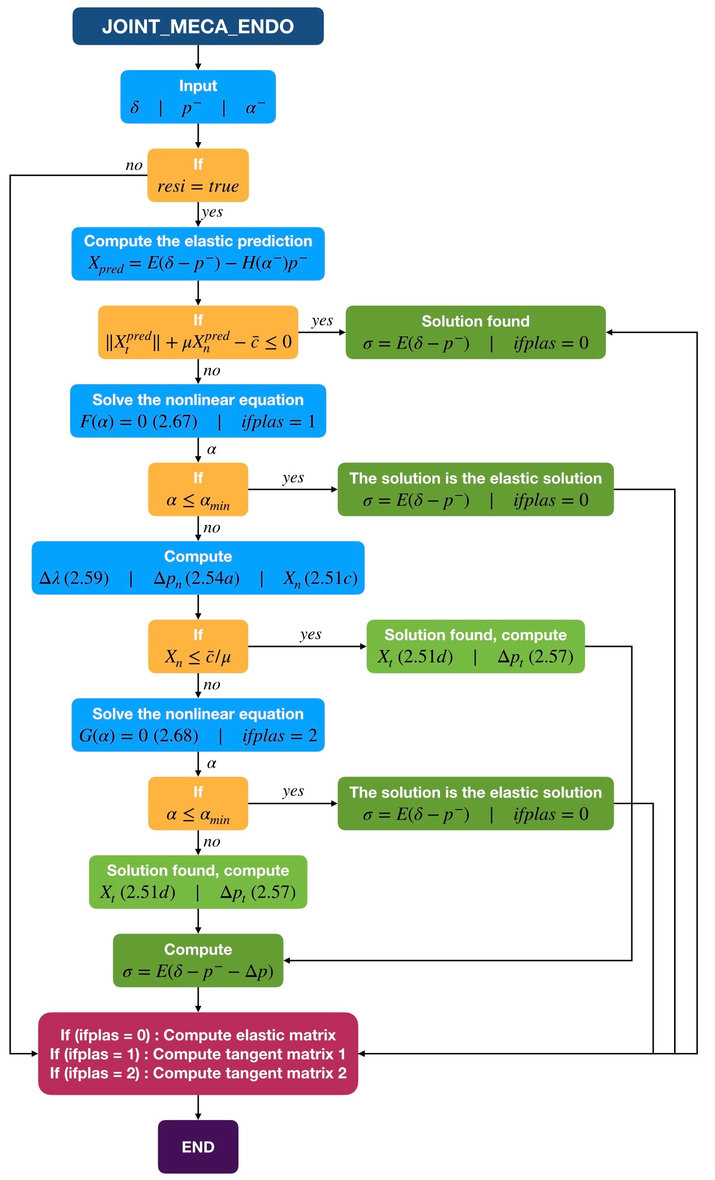
This equation system is solved by the standard elastic prediction procedure. In the damaging plastic phase, we obtain an implicit equation system with the following four unknowns \(\mathrm{\Delta }{p}_{n};\mathrm{\Delta }\vec{{p}_{t}};\mathrm{\Delta }\mathrm{\lambda };\mathrm{\Delta }\mathrm{\alpha }\). Using the fact that \(\mathrm{\Delta }\vec{{p}_{t}}\uparrow \uparrow {K}_{t}(\vec{{\mathrm{\delta }}_{t}}-{\vec{p}}_{t}^{\text{-}})-{A}_{t}({\mathrm{\alpha }}^{\text{+}})\cdot {\vec{p}}_{t}^{\text{-}}\) the system can be simplified is brought back to an equation for the single scalar unknown \({\mathrm{\alpha }}^{\text{+}}={\mathrm{\alpha }}^{\text{-}}+\mathrm{\Delta }\mathrm{\alpha }\). For this purpose, the unknown \(\mathrm{\Delta }\mathrm{\lambda }\) is expressed using the two threshold functions. From the plastic threshold we get:

(4.7)#\[ \ mathrm {\ Delta}\ mathrm {\ lambda} =\ frac {\ vert {K} _ {t} (\ vec {\ mathrm {\ delta}} _ {t}} - {\ vec {p}}} - {\ vec {p}}} _ {p}} _ {\ text}}) - {\ text {-}} ({\ mathrm {\ alpha}}} - {\ vec {p}}} - {\ vec {p}}} - {\ vec {p}}} - {\ vec {p}}} _ {p}} - {\ vec {p}}} _ {p}} - {\ vec {p}}} _ {p}} - {\ vec {p}}} _ {p}} - {\ vec {p}}} +}})\ cdot {\ vec {p}} _ {t}} _ {t}} ^ {\ text {-}}\ green +\ mathrm {\ mu} {K} _ {n} ({\ mathrm {\ delta}}} _ {n}} _ {p} ^ {\ text {-}}}) -\ mathrm {\ mu} {n} ({\ delta}}} ({\ mathrm {\ delta}}}} _ {delta}}} ({\ delta}}} _ {delta}}} _ {delta}}} _ {delta}}} _ {delta}}} _ {delta}}} _ {delta}}} _ {delta}}} _ {delta}}} _ {delta}}} _ {delta}}} _ {delta}} mathrm {\ alpha}} ^ {\ text {+}})\ cdot {+}})\ cdot {p}} _ {n} ^ {\ text {-}} -\ overline {c}} {{\ mathrm {\ mu}}}} ^ {\ mu}}}} ^ {\ mu}}} {\ mathrm {\ mu}}} {\ mu}} {\ mu}} {\ mu}}} ^ {\ mu}}} ^ {\ mu}}} ^ {\ mu}}} ^ {\ mu}}} ^ {\ mu}}} ^ {\ mu}}} ^ {\ mu}}} ^ {\ mu}}} ^ {\ mu}}} ^ {\ mu}}} ^ {\ mu}}} ^ {\ mu}}} ({\ mathrm {\ alpha}}} ^ {\ text {+}}}) + {A} _ {t} ({\ mathrm {\ alpha}}} ^ {\ text {+}}})} ^ {\ text {+}})}\]

In parallel, starting from the damage threshold, we have:

(4.8)#\[\begin{split} \ begin {array} {c} F ({\ mathrm {\ alpha}}} ^ {\ text {+}}) =- ({\ mathrm {\ mu}} ^ {2} {B} _ {n} + {n} + {B}} + {B} _ {t})\ mathrm {\ alpha}} ^ {2} -2\ left (\ mathrm {\ alpha}}) ^ {2} {B}} + {n} + {B} + {B} _ {t}) + {B} _ {t})\ mathrm {\ t})\ mathrm {\ delta} {\ lambda}} ^ {2}} -2\ left (\ mathrm {\ lambda}} ^ {2} -2\ left (\ mathrm {\ alpha} mu} {B} _ {n} + {B} _ {t} {t} {\ vec {p}}} _ {t} ^ {\ text {-}}\ frac {{K} _ {t} (\ vec {{\ mathrm {\ mathrm {\ delta}}} _ {delta}}} _ {t}} - {t}} - {\ vec {p}}} _ {t}}) - {a} _ {t}) - {A} _ {t}} (\ vec {\ mathrm {\ delta}}} _ {t}} ({\ mathrm {\ alpha}}} ^ {\ text {+}})\ cdot {\ vec {+}}})\ cdot {\ vec {p}}} {\ green {K} _ {t} (\ vec {\ text {+}}})\ cdot {\ text {+}}})\ cdot {\ vec {p}}}} {\ text {-}}} {\ vert {K} _ {t}} {t}} {\ vert {K} _ {t}} (\ vec {-}}) (\ vec {\ text {-}}) (\ vec {\ text {-}}) (\ vec {\ text {-}}) (\ vec {\ text {-}}) (\ vec {\ text {-}}) (\ vec {A} _ {t} ({\ mathrm {\ alpha}}} ^ {\ text {+}}})\ cdot {\ vec {p}} _ {t} ^ {\ text {-}}\ green}\ right)\ mathrm {\ alpha}}\ right)\ mathrm {\ Delta}}\\\ - {b} ^ {b} {p} {p}\ right)\ mathrm {\ Delta}}\ delta}\ mathrm {\ Delta}\\}\ {\ text {-} 2} - {B} _ {t} {\ vec {p}} _ {t} ^ {\ ^ {\ text {-} 2} -\ frac {2 {D} _ {1}}} {S\ text {'} ({\ mathrm {\ alpha}}} ^ {\ text {+}}})})} =0\ end {array}}\end{split}\]

Substituting \(\mathrm{\Delta }\mathrm{\lambda }\) from EQ. into Eq., we get a non-linear scalar equation for \({\mathrm{\alpha }}^{\text{+}}\). This non-linear equation is solved by the desiccation method alternated with the rope method.

The same set of equations is solved in the tip of the cone by adopting the flow rule according to the outgoing normals:

(4.9)#\[ G ({\ mathrm {\ alpha}}} ^ {\ text {+}}) =- {\ text {+}}) =- {B} _ {n} {\ mathrm {\ delta}} _ {\ delta}} _ {n}} _ {n}} _ {n}} _ {n}} _ {n}} _ {n}} _ {n}} _ {n}} _ {n}} _ {n}} _ {n}} _ {n}} _ {n}} _ {n}} _ {n}} _ {n}} _ {n}} _ {n}} _ {n}} _ {n}} mathrm {\ alpha}} ^ {\ text {+}})}}\ right)}}\ right)}}\ right)}} ^ {2} - {B} _ {\ left (\ frac {{K} _ {t}}\ vec {{\ mathrm {+}}} {\ mathrm {\ delta}}} _ {t}}\ vec {{\ mathrm {\ delta}}} _ {t}} ^ {\ text {+}})}\ right)}\ right)}} ^ {2} -\ frac {2 {D} _ {1}} {S\ text {'}} ({\ mathrm {\ alpha}}}}} ^ {\ text {+}}})} =0\]

The resolution algorithm is summarised schematically as follows:

4.2. Internal variables#

Law JOINT_MECA_ENDO has eighteen internal variables. From the point of view of the law of behavior, only the first, the third, and the fourth are*stricto sensu* internal variables. The others provide information on the hydromechanical state of the joint at a given moment.

\(V1\)	Increasing parameter indicating the cumulative plasticity during sliding \(\mathrm{\lambda }\).
\(V2\)	Slip indicator \(=0\) if the regime is linear elastic, \(=1\) if the regime is plastic in shear under compression, \(=2\) if the regime is plastic in tension.
\(V3\)	Normal lamination at joint orientation \({p}_{n}\) [12] _
\(V4\) \(V5\)	Tangential plasticization vector \(\vec{{p}_{t}}\). \(V5\) is set to zero in 2D.
\(V6\)	Damage variable \(\mathrm{\alpha }\mathrm{:}0\le \mathrm{\alpha }\le 1\).
\(V7\)	Normal \(\mathit{V7}={\delta }_{n}\) jump in the local coordinate system.
\(V8\) \(V9\)	Tangential jump \({\mathrm{\delta }}_{t1}\) and \({\mathrm{\delta }}_{t2}\) in the local coordinate system (\(V9\) null in 2D).
\(V10\)	Unused variable (reserved for future changes to the law).
\(V11\)	Normal mechanical stress \({\mathrm{\sigma }}_{n}\) (without fluid pressure).
\(V12\) \(V13\) \(V14\)	Components of the pressure gradient in the global coordinate system (only for modelsxxx_ JOINT_HYME). \({\partial }_{x}p\), \({\partial }_{y}p\), and \({\partial }_{z}p\) respectively.
\(V15\) \(V16\) \(V17\)	Hydraulic flow components in the global coordinate system (only for xxx_ JOINT_HYME models). \({w}_{x}\), \({w}_{y}\), and \({w}_{z}\) respectively.
\(V18\)	User imposed fluid pressure \(p\) (PRES_FLUIDE) in the case of models xxx_ JOINTou fluid pressure interpolated from that calculated at the middle nodes of the joint elements (degree of freedom of the problem) for the models: xxx_ JOINT_HYME.
\(V19\) \(V20\)	Tangential mechanical stresses \({\mathrm{\sigma }}_{t1}\) and \({\mathrm{\sigma }}_{t2}\) (\(V20\) zero in 2D).