6. Validation#
The first step in validating the model is comparing the prediction with various experimental results for simple tests. Given the simplifying hypotheses that were made for our modeling, we will of course not be able to reproduce all the experiments, in particular the triaxial compression experiments. The focus here is on simple tension tests, simple compression tests, as well as biaxial tests.
6.1. Identifying parameters#
The identification of the parameters must be done in three successive phases:
A value must be selected for the coupling constant \(\alpha\). It must be taken in such a way that scalar compression damage remains negligible in a tensile test. We decided to take it equal to \(\mathrm{0,87}\) for all the tests in this section in order to avoid the phenomenon of snap-back in compression (see [§ 4.1.2]).
The second phase is the identification of parameters \({k}_{0}\) and \({\gamma }_{B}\). These parameters can be identified directly on the simple tensile test because the other parameters of the model are not involved in this test.
The third phase is the identification of parameters \({\gamma }_{d}\), \({k}_{1}\) and \({k}_{2}\) on simple compression tests and biaxial tests.
In all rigor, the identification of the parameters of our model for a material requires the availability of experimental curves in simple tension, in simple compression and under biaxial loading. Unfortunately, all of these results are generally not available simultaneously for a material. We will therefore have to make a certain number of assumptions to calibrate our parameters. For example, we will choose parameter \({k}_{2}\) for all tests in such a way that the tensile stresses in the biaxial tests do not exceed the tensile breaking stress. In addition, we do not have the tensile breaking stress for compression tests for the materials studied. We will therefore arbitrarily take parameters \({k}_{0}\) and \({\gamma }_{B}\) equal to those we calculated for the simple tensile test.
6.2. Simple traction#
Experiments to observe the behavior of concrete under tensile loading are extremely difficult to perform, which explains the relatively low number of simple tensile test results. The difficulty lies in the fact that the damage is concentrated in localization bands corresponding to cracks, which has the effect of making the specimen under study inhomogeneous. As soon as strong heterogeneities appear, it becomes impossible to deduce a stress-strain curve from the force-displacement curve, and therefore to establish a law of behavior for the material. The measuring device PIED ([bib6], [bib7]) makes it possible to measure a relatively homogeneous stress and deformation field by limiting the location. That is why we use the results obtained by [bib6] to test our model.
In the case of simple traction, only 3 of the 6 parameters of the model will play a role:
The coupling parameter \(\alpha\).
Threshold constant \({k}_{0}\).
The blocked energy constant associated with traction damage \({\gamma }_{B}\).
Parameters \({k}_{1}\) and \({k}_{2}\) have no influence on this test and the influence of parameter \({\gamma }_{d}\) is negligible.
Parameter \({k}_{0}\) controls the height of the stress peak and parameter \({\gamma }_{B}\) controls its width as well as the post-peak slope. The greater \({\gamma }_{B}\), the less rapidly the damage evolves, which causes non-linearity to appear before the peak and increases the deformation at the peak and its width. The [Figure 6.2-a] shows the response of the model, compared to the experimental data from [bib6]. The calculation is carried out on a single element so as not to encounter a localization phenomenon. The settings are as follows:
\(\alpha\) |
|
\({\gamma }_{B}\) (\(\mathit{kJ}\mathrm{/}{m}^{3}\)) |
0.87 |
3.10-4 |
7 |
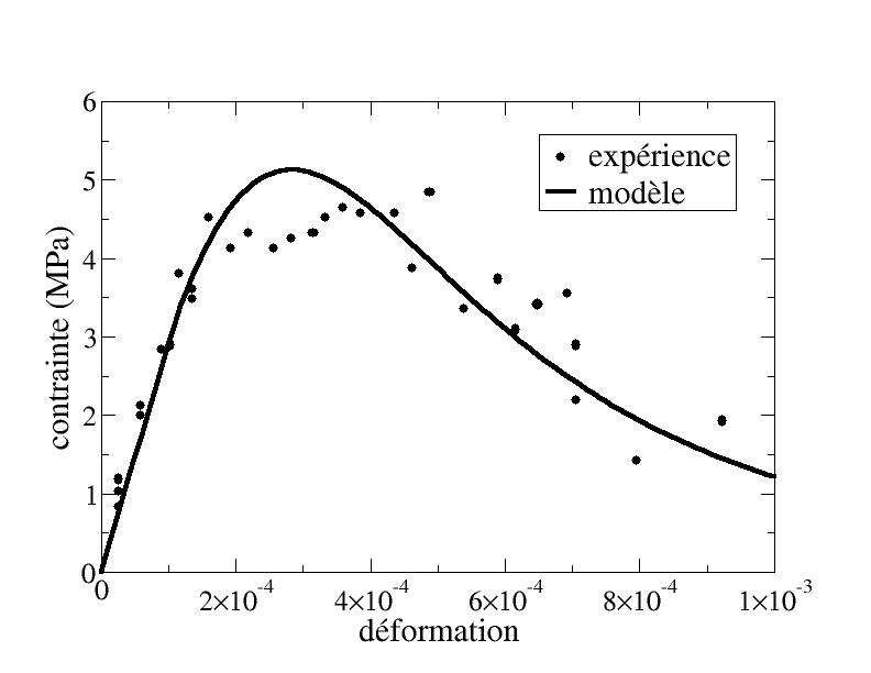
Figure 6.2-a: Simple tensile test, comparison with experimental data from Bazant and Pijaudier-Cabot [1989]
6.3. Simple compression#
The fact that the experimental data is more numerous than for the tensile tests is due to the fact that they are easier to perform. The localization phenomenon is much less important there than for traction loading, at least when the damage remains relatively low. We use the results of Hognestad et al. [bib8] and the Ramtani test [bib9] to validate our model on simple compression tests. Despite the fact that the results of [bib8] are relatively old, we use them because the experiment was conducted for several different types of concrete. We also use the results of [bib9] to show that the model is still valid for more recent experiments.
As we said in paragraph [§ 6.1], we do not have the tensile breaking stress for these various tests, which is why we use the same parameters as those obtained in paragraph [§ 6.2]: \(\alpha =\mathrm{0,87},{k}_{0}={3.10}^{-4}\mathrm{MPa},{\gamma }_{B}=7\mathrm{kJ}/{m}^{\text{}}\).
6.3.1. Hognestad et al. [1955]#
The [Figure 6.3.1-a] shows us the comparison between the experimental results of [bib8] and the prediction of our model in the case of three materials whose maximum stress in absolute value is noted \({f}_{c}\):
We used the following settings:
Ultimate constraint \({f}_{c}\) |
|
|
|
|
\(E\) |
17000 |
27000 |
36000 |
|
\(\nu\) |
0.2 |
0.2 |
0.2 |
|
\({\gamma }_{d}\) (\(\mathrm{kJ}/{m}^{3}\)) |
60 |
60 |
60 |
|
\({k}_{1}\) (\(\mathrm{MPa}\)) |
4.8 |
18 |
||
\({k}_{2}\) |
7.10-4 |
7.10-4 |
7.10-4 |
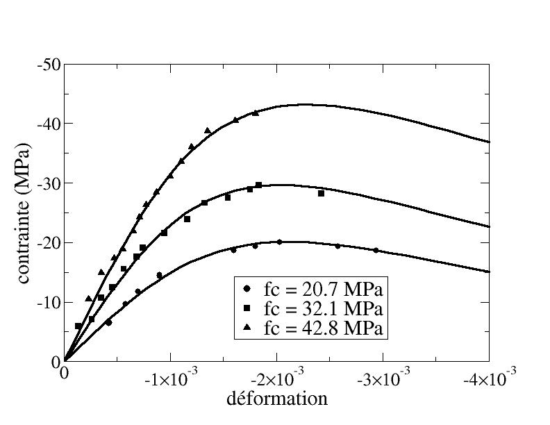
Figure 6 .3.1-a: Simple compression tests by Hognestad et al. [1955]
6.3.2. Ramtani [1990]#
The [bib9] test is a cyclic compression test. It highlights the creation of irreversible deformations and the phenomenon of hysteresis. We do not describe these phenomena. For our part, we are therefore content to calculate the response under monotonic loading. The parameters used are as follows:
\(E\) |
|
|
\({k}_{1}\) (\(\mathrm{MPa}\)) |
\({k}_{2}\) |
|
33700 |
0.2 |
60 |
60 |
20.5 |
7.10-4 |
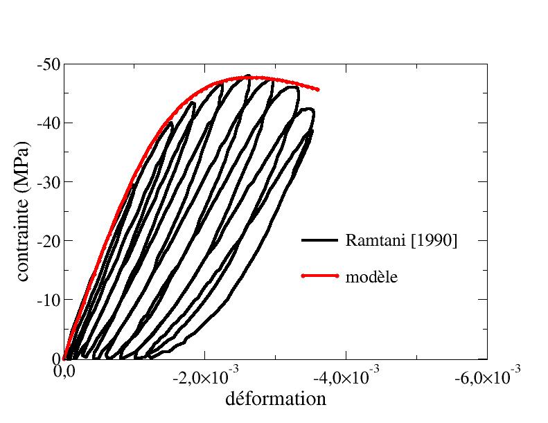
Figure 6 .3.2-a: Ramtani simple compression tests [1990]
6.4. Simple traction followed by simple compression#
We propose here to compare our model to the experimental results of [bib9] on a simple tensile test followed by a simple compression, in order to demonstrate the restoration of stiffness caused by the reclosing of cracks.
The parameters used are as follows:
The experimental results show the appearance of irreversible deformations in the simple traction phase (cf. [Figure 6.4-a]). These irreversible deformations are not described by our model, which is why the loss of stiffness caused by the damage seems overestimated. This problem does not seem to have an impact when the cracks close. Indeed, on the [Figure 6.4-b], a good correspondence of the model with the experimental results in the compression phase is observed. It thus seems that the restoration of the stiffness obtained thanks to the model is very close to that obtained experimentally.
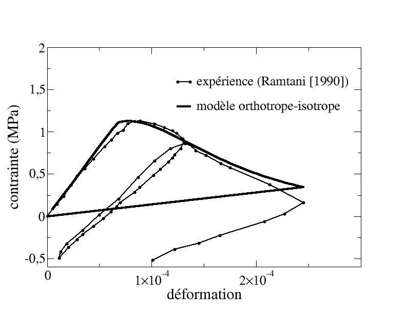
Figure 6 .4-a: Simple traction phase in the Ramtani test [1990]
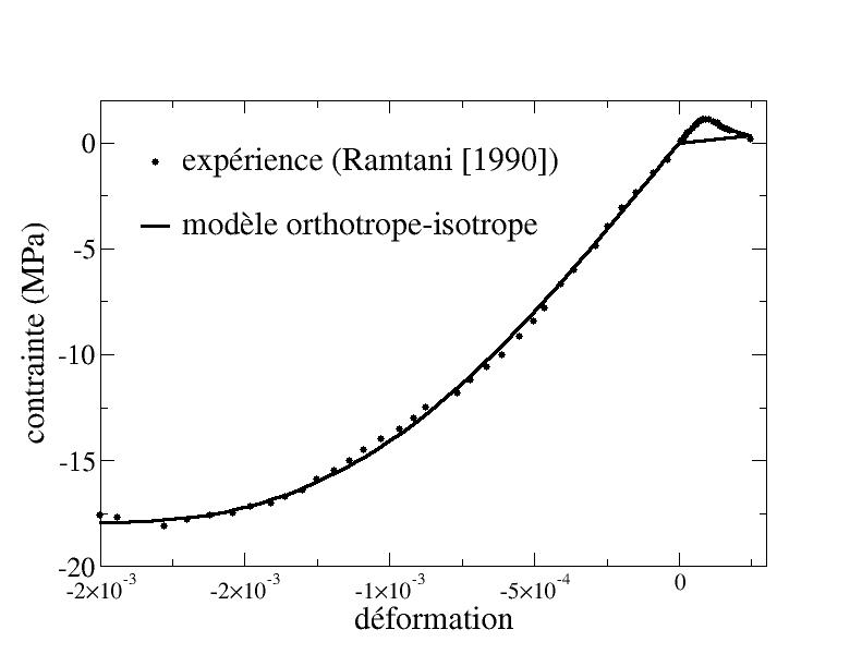
Figure 6 .4-b: Tensile tests followed by simple compression (Ramtani [1990])
6.5. Biaxial tests#
This paragraph is devoted to the study of the biaxial tests of [bib5]. On the one hand, the aim is to observe the stress-deformation response in the case of uniaxial loading and two biaxial loads under plane stress, and on the other hand to describe the envelope of the fracture domain in the stress space in the case of biaxial loads under plane stresses.
Note:
The experiences of [bib5] are relatively old. These biaxial tests require a large number of tests, which is why there are few more recent results on this type of test. We use them because they always represent a reference for modellers.
The maximum stress in absolute value of uniaxial compression, noted \({\beta }_{p}\) in [bib5], is equal to 4650 \(\mathrm{psi}\) (32.1 \(\mathrm{MPa}\)). We normalize our response by this breaking stress. The settings we use are as follows:
6.5.1. Stress-strain response#
First, the stress-strain response is plotted in the case of uniaxial loading and two biaxial loads under plane stress:
\({\mathrm{\sigma }}_{2}={\text{\eta \sigma }}_{1}\) with \(\eta =(\mathrm{0,0}.52\mathrm{,1})\) and \({\mathrm{\sigma }}_{3}=0\).
The model allows us to obtain the answers represented [Figure 6.5.1-b] which we compare to the results of [bib5] represented [Figure 6.5.1-a]. As we saw in the preceding paragraph, it is possible to correctly describe the uniaxial compression behavior in the compression direction. However, we can see for this test that the lateral deformation predicted by the model decreases when the damage occurs when it actually increases. This is due to the fact that the existence of irreversible damage-dependent deformations, which seem to be at the origin of volume expansion under compression, was not taken into account. This phenomenon is even more important in the case of bicompression tests. In fact, it is observed with the model that the fracture threshold in bicompression is higher than that in simple compression (less than the experimental results), but that the deformations at break are less important in the case of bicompression than for compression, which does not correspond to the experimental results.
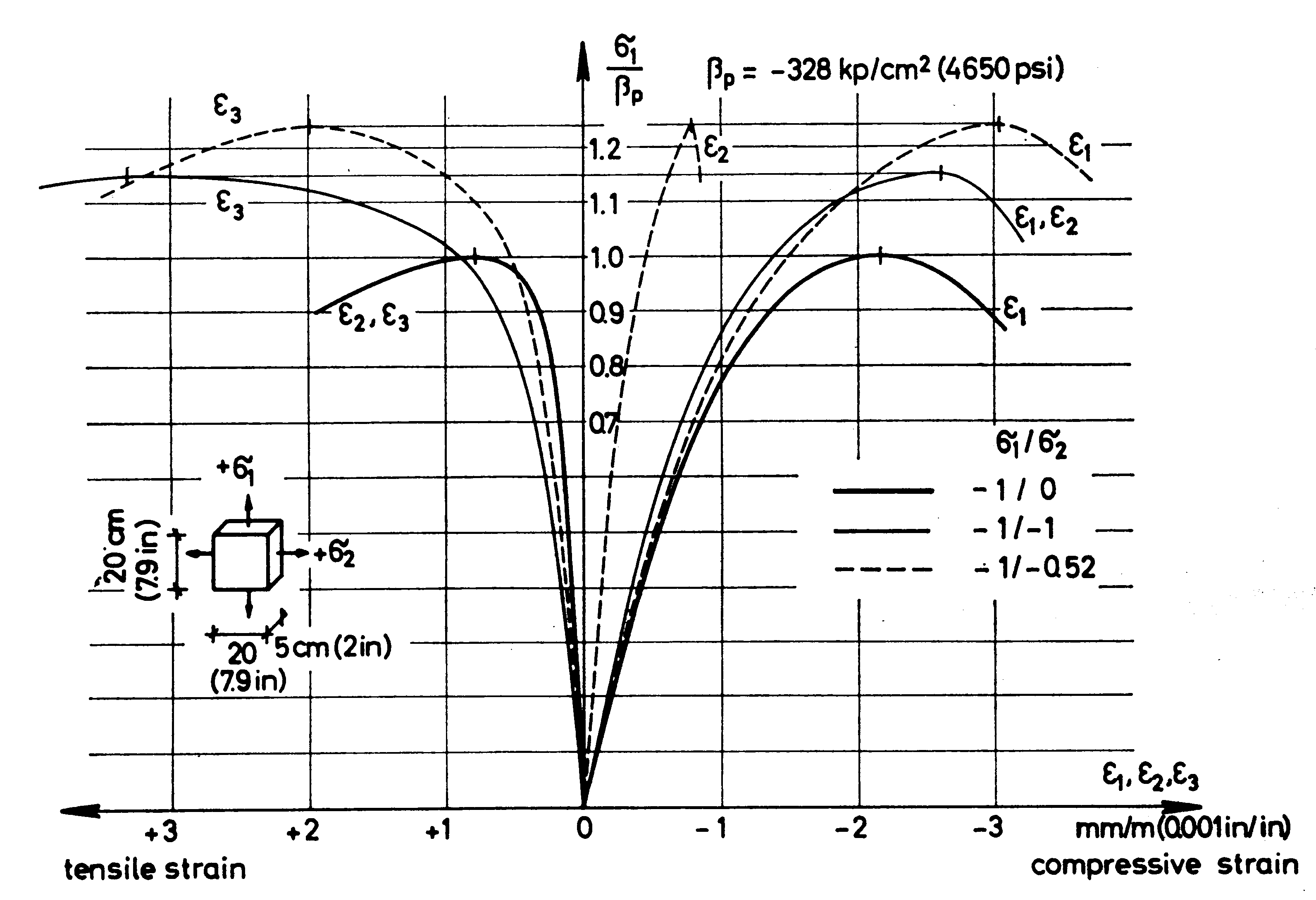
Figure 6.5.1-a: Biaxial assays by Kupfer et al. [1969]
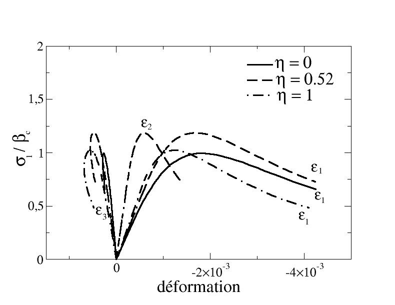
Figure 6.5.1-b: Model response for biaxial tests
6.5.2. Rupture domain envelope#
We are now interested in the envelope of the fracture domain for biaxial tests under plane stress. The experimental results obtained by [bib5] for various concretes are represented on [Figure 6.5.2-a]. A relative similarity in the shape of the standardized rupture envelope is observed for the various materials.
We used the parameters used in paragraph [§ 6.5.1] and we compared the prediction of our model for the rupture envelope of biaxial tests with the experimental results (cf. [Figure 6.5.2-b]).
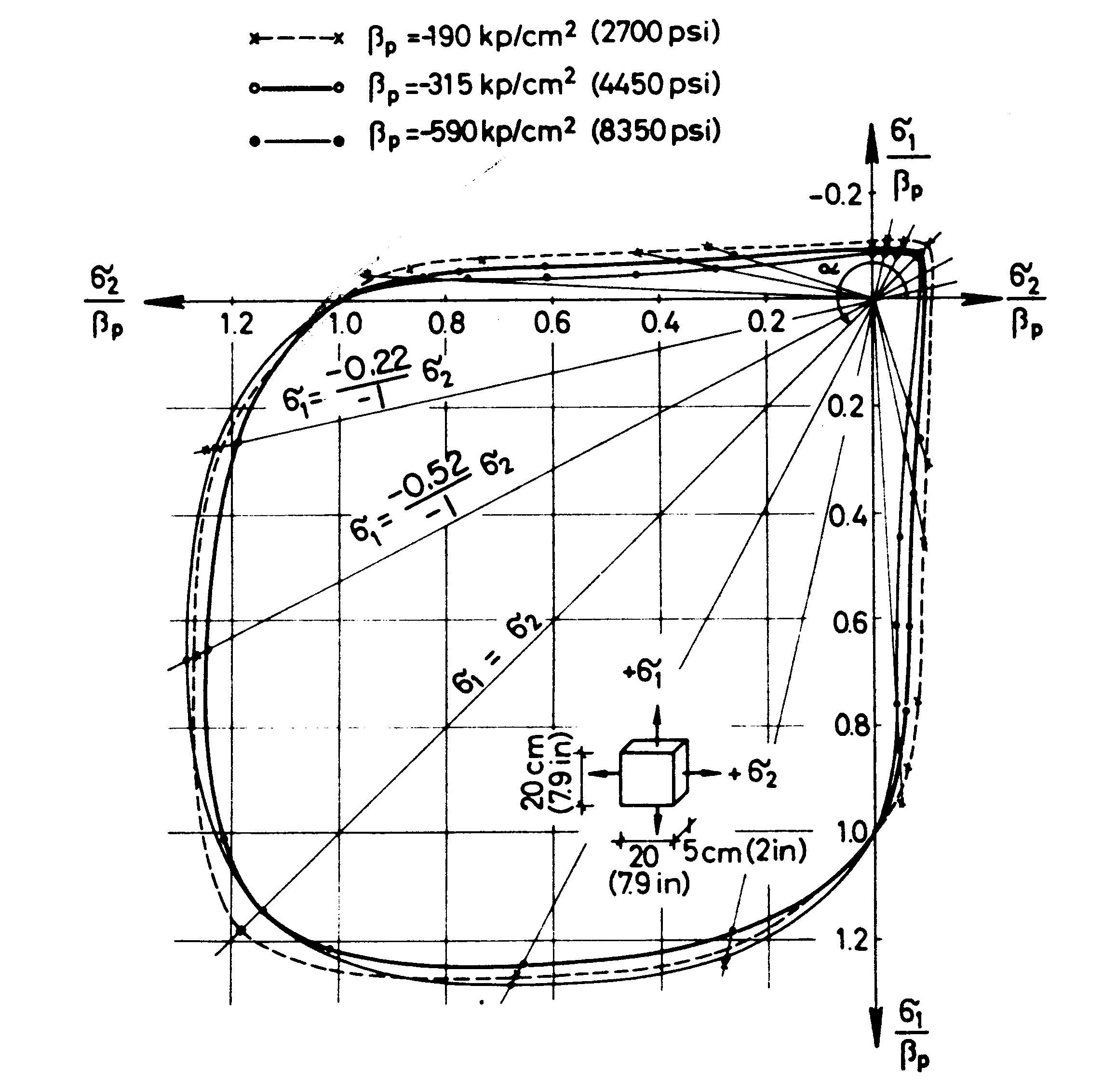
Figure 6.5.2-a: Fracture envelope for biaxial tests under plane stresses Kupfer et al. [1969]
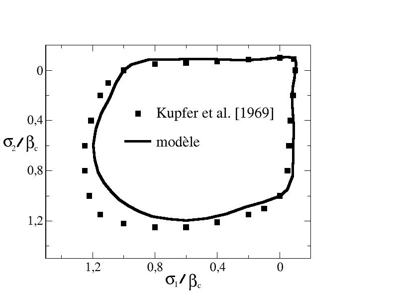
Figure 6.5.2-b: Model prediction for the rupture envelope biaxial tests under planar stres
A relatively satisfactory correspondence between the prediction and the experimental results is observed. The biggest gap is in the bicompression zone. This problem is not surprising insofar as we decided to use only two parameters for the threshold, which control the shape of the rupture envelope as well as the response of the model under compression. A more thorough study of the threshold function would probably make it possible to better approach the experimental results, at the cost of introducing new parameters.
A1.1 Definition of spectral decomposition and the positive and negative parts of a tensor
Let \(X\) be a symmetric tensor of order 2. To avoid making the ratings heavier, we will also write \(X\), abusively, the matrix of this tensor in the observer’s fixed base. In addition, let \(\tilde{X}\) be the matrix (diagonal) of this tensor in its own base:
\(\tilde{X}=(\begin{array}{ccc}{\tilde{X}}_{1}& 0& 0\\ 0& {\tilde{X}}_{2}& 0\\ 0& 0& {\tilde{X}}_{3}\end{array})\) eq A1.1-1
By noting \({U}_{i}\) the eigenvector associated with the th eigenvalue, and \(Q=({U}_{1},{U}_{2},{U}_{3})\) the transition matrix between the fixed base and the eigenbase of \(X\), we have the relationship:
\(X=Q\text{.}\tilde{X}\text{.}{Q}^{T}\) eq A1.1-2
The positive and negative parts of tensor \(X\) are defined by:
\({X}_{+}={P}_{+}:X=Q\text{.}{\tilde{X}}_{+}\text{.}{Q}^{T}\) with \({\tilde{X}}_{+}=(\begin{array}{ccc}H({\tilde{X}}_{1}){\tilde{X}}_{1}& 0& 0\\ 0& H({\tilde{X}}_{2}){\tilde{X}}_{2}& 0\\ 0& 0& H({\tilde{X}}_{2}){\tilde{X}}_{3}\end{array})\) eq A1.1-3
\({X}_{-}={P}_{-}:X=Q\text{.}{\tilde{X}}_{-}\text{.}{Q}^{T}\) with \({\tilde{X}}_{-}=(\begin{array}{ccc}H(-{\tilde{X}}_{1}){\tilde{X}}_{1}& 0& 0\\ 0& H(-{\tilde{X}}_{2}){\tilde{X}}_{2}& 0\\ 0& 0& H(-{\tilde{X}}_{2}){\tilde{X}}_{3}\end{array})\) eq A1.1-4
where \(H\) is the Heaviside function.
A1.2 Calculation of derivatives
To calculate the tangent matrix, as well as to calculate the evolution of damage, we need to evaluate the derivative of the positive and negative parts of a tensor with respect to the latter. To do this, simply imagine that the tensor \(X\) depends on time and to calculate the tensors \({M}_{+}\) and \({M}_{-}\) defined by:
\({\dot{X}}_{+}={M}_{+}:\dot{X}\) and \({\dot{X}}_{-}={M}_{-}:\dot{X}\) eq A1.2-1
Differentiating equation [éq A1.1-2] gives us:
\({\dot{X}}_{+}=Q\text{.}{\tilde{\dot{X}}}_{+}\text{.}{Q}^{T}+\dot{Q}\text{.}{\tilde{X}}_{+}\text{.}{Q}^{T}+Q\text{.}{\tilde{X}}_{+}\text{.}{\dot{Q}}^{T}\) eq A1.2-2
Hypothesis:
We need to establish the expression of \(\dot{Q}\). The following demonstration is only valid if the eigenvalues of \(X\) are distinct. Since the calculation of \({M}_{+}\) and \({M}_{-}\) will only be used in numerical resolution algorithms, we will allow ourselves to numerically disturb any identical eigenvalues in order to make them distinct and to be able to use the results below.
To calculate \(\dot{Q}\), we need to express the derivative of the eigenvectors \({\dot{U}}_{i}\). To do this, according to the approach of [bib11], we differentiate the expression from \(X\):
\(X=\sum _{i}{\tilde{X}}_{i}{U}_{i}\otimes {U}_{i}\Rightarrow \dot{X}=\sum _{i}{\tilde{\dot{X}}}_{i}{U}_{i}\otimes {U}_{i}+{\tilde{X}}_{i}{\dot{U}}_{i}\otimes {U}_{i}+{\tilde{X}}_{i}{U}_{i}\otimes {\dot{U}}_{i}\) eq A1.2-3
In addition, we have the following relationships between the eigenvectors and their derivatives:
\({U}_{i}\text{.}{U}_{j}={\mathrm{\delta }}_{\text{ij}}\) , \({\dot{U}}_{i}\text{.}{U}_{j}+{U}_{i}\text{.}{\dot{U}}_{j}=0\) eq A1.2-4
By contracting equation [éq A1.2-3] left and right by the eigenvectors, and using the relationships [éq A1.2-4], we get the following relationships:
\({U}_{i}\text{.}\dot{X}\text{.}{U}_{i}\Rightarrow {(\dot{\tilde{X}})}_{\text{ii}}={\tilde{\dot{X}}}_{i}\) eq A1.2-5
\({U}_{j}\text{.}\dot{X}\text{.}{U}_{k}\Rightarrow {(\dot{\tilde{X}})}_{\text{jk}}={\tilde{X}}_{k}{U}_{j}\text{.}{\dot{U}}_{k}+{\tilde{X}}_{j}{\dot{U}}_{j}\text{.}{U}_{k}=({\tilde{X}}_{j}-{\tilde{X}}_{k}){\dot{U}}_{j}\text{.}{U}_{k}\text{pour}j\ne k\) eq A1.2-6
In these expressions, there is no summation on the indices, \({(\dot{\tilde{X}})}_{\text{jk}}\) designate the components of \(\dot{X}\) in the fixed base coinciding with the eigenbase of \(X\) at the time in question \(({(\dot{\tilde{X}})}_{\text{jk}}={U}_{j}\text{.}\dot{X}\text{.}{U}_{k})\), and the \({\tilde{\dot{X}}}_{i}\) designate the derivatives of the eigenvalues of \(X\) (not the eigenvalues of the derivative \(\dot{X}\)).
We deduce from the relationship [éq A1.2-6] the expression for \({\dot{U}}_{j}\):
\({\dot{U}}_{j}=\sum _{k\ne j}({\dot{U}}_{j}\text{.}{U}_{k})\text{.}{U}_{k}=\sum _{k\ne j}\frac{{(\dot{\tilde{X}})}_{\text{jk}}}{({\tilde{X}}_{j}-{\tilde{X}}_{k})}{U}_{k}\) eq A1.2-7
This allows us to express \(\dot{Q}\):
\(\dot{Q}=({\dot{U}}_{1},{\dot{U}}_{2},{\dot{U}}_{3})\Rightarrow {\dot{Q}}_{\text{ij}}=\sum _{k\ne j}\frac{{(\dot{\tilde{X}})}_{\text{jk}}}{({\tilde{X}}_{j}-{\tilde{X}}_{k})}{Q}_{\text{ik}}\) eq A1.2-8
The \({(\dot{\tilde{X}})}_{\text{jk}}\), components of \(\dot{X}\) in the fixed base coinciding with the eigenbase of \(X\) at the time in question, can be expressed as a function of the components of \(\dot{X}\) in the fixed base. So, \(\dot{\tilde{X}}\) designating the \({(\dot{\tilde{X}})}_{\text{jk}}\) matrix, we have:
\(\dot{\tilde{X}}={Q}^{T}\text{.}\dot{X}\text{.}Q\) eq A1.2-9
From the expression [éq A1.2-8] we deduce the expression for \(\dot{Q}\):
\({\dot{Q}}_{\text{ij}}=\sum _{k\ne j}\sum _{m,n}\frac{{Q}_{\text{mj}}{Q}_{\text{nk}}{\dot{X}}_{\text{mn}}}{({\tilde{X}}_{j}-{\tilde{X}}_{k})}{Q}_{\text{ik}}\) eq A1.2-10
We finally have the obvious relationships between the eigenvalues of \({X}_{+}\) and \(X\):
\({\tilde{X}}_{+{}_{i}}=H({\tilde{X}}_{i}){\tilde{X}}_{i}\Rightarrow {\tilde{\dot{X}}}_{+{}_{i}}=H({\tilde{X}}_{i}){\tilde{\dot{X}}}_{i}\) eq A1.2-11
From the relationships [éq A1.2-5], [éq A1.2-9] and [éq A1.2-11], we deduce the following relationship:
\({\tilde{\dot{X}}}_{+{}_{i}}=H({\tilde{X}}_{i}){\tilde{\dot{X}}}_{i}=H({\tilde{X}}_{i}){(\dot{\tilde{X}})}_{\text{ii}}=H({\tilde{X}}_{i}){Q}_{\text{ji}}{Q}_{\text{ki}}{\dot{X}}_{\text{jk}}\) eq A1.2-12
The relationships [éq A1.2-10], [éq A1.2-11], and [éq A1.2-12] allow us to express the relationship [éq A1.2-2]:
\({\dot{X}}_{+{}_{\text{ij}}}=\sum _{k,l}\left[\sum _{m}{Q}_{\text{im}}{Q}_{\text{jm}}{Q}_{\text{km}}{Q}_{\text{lm}}H({\tilde{X}}_{m})\right]{\dot{X}}_{\text{kl}}+\sum _{k,l}\left[\sum _{\begin{array}{}m\ne n\\ m,n\end{array}}\frac{{Q}_{\text{km}}{Q}_{\text{ln}}}{\tilde{{X}_{m}}-\tilde{{X}_{n}}}H(\tilde{{X}_{m}})\tilde{{X}_{m}}({Q}_{\text{in}}{Q}_{\text{jm}}+{Q}_{\text{im}}{Q}_{\text{jn}})\right]{\dot{X}}_{\text{kl}}\)
eq A1.2-13
Since \(X\) is a symmetric tensor, we have:
\(X=\frac{1}{2}(X+{X}^{T})\Rightarrow \dot{X}=\frac{1}{2}(\dot{X}+{\dot{X}}^{T})\) eq A1.2-14
This allows us to rewrite equation [éq A1.2-13]:
\(\begin{array}{}{\dot{X}}_{+{}_{\text{ij}}}=\sum _{k,l}\left[\sum _{m}{Q}_{\text{im}}{Q}_{\text{jm}}{Q}_{\text{km}}{Q}_{\text{lm}}H({\tilde{X}}_{m})\right]{\dot{X}}_{\text{kl}}\\ +\frac{1}{2}\sum _{k,l}\left[\sum _{\begin{array}{}m\ne n\\ m,n\end{array}}({Q}_{\text{km}}{Q}_{\text{ln}}+{Q}_{\text{kn}}{Q}_{\text{lm}})\frac{H(\tilde{{X}_{m}})\tilde{{X}_{m}}}{\tilde{{X}_{m}}-\tilde{{X}_{n}}}({Q}_{\text{in}}{Q}_{\text{jm}}+{Q}_{\text{im}}{Q}_{\text{jn}})\right]{\dot{X}}_{\text{kl}}\end{array}\) eq A1.2-15
From this we deduce the expression for the components of \({M}_{+}\):
\({M}_{\text{+ijkl}}=\sum _{m}{Q}_{\text{im}}{Q}_{\text{jm}}{Q}_{\text{km}}{Q}_{\text{lm}}H({\tilde{X}}_{m})+\frac{1}{2}\sum _{\begin{array}{}m\ne n\\ m,n\end{array}}({Q}_{\text{km}}{Q}_{\text{ln}}+{Q}_{\text{kn}}{Q}_{\text{lm}})\frac{H(\tilde{{X}_{m}})\tilde{{X}_{m}}}{\tilde{{X}_{m}}-\tilde{{X}_{n}}}({Q}_{\text{in}}{Q}_{\text{jm}}+{Q}_{\text{im}}{Q}_{\text{jn}})\) eq A1.2-16
By analogy, we can easily deduce the expression for the components of \({M}_{-}\):
\({M}_{\text{-ijkl}}=\sum _{m}{Q}_{\text{im}}{Q}_{\text{jm}}{Q}_{\text{km}}{Q}_{\text{lm}}H({\tilde{-X}}_{m})+\frac{1}{2}\sum _{\begin{array}{}m\ne n\\ m,n\end{array}}({Q}_{\text{km}}{Q}_{\text{ln}}+{Q}_{\text{kn}}{Q}_{\text{lm}})\frac{H(\tilde{-{X}_{m}})\tilde{{X}_{m}}}{\tilde{{X}_{m}}-\tilde{{X}_{n}}}({Q}_{\text{in}}{Q}_{\text{jm}}+{Q}_{\text{im}}{Q}_{\text{jn}})\) eq A1.2-17
We want to show that when an eigenvalue of the damage reaches 1 in one direction, then this direction is blocked and the damage can only evolve in the plane orthogonal to this direction.
We place ourselves in the clean base of the damage:
\(D=\sum _{i}{\tilde{D}}_{i}{e}_{i}\otimes {e}_{i}\) eq A2-1
where \({e}_{i}\) refers to the eigenvector associated with the eigenvalue \({\tilde{D}}_{i}\).
The energy adopted is the sum of an elastic energy and a function indicative of the eigenvalues of the damage:
\(\mathrm{\varphi }(\mathrm{\varepsilon },D)={\mathrm{\varphi }}^{\text{el}}(\mathrm{\varepsilon },D)+{I}_{]-\infty \mathrm{,1}]}\left[\text{max}({\tilde{D}}_{i})\right]\) eq A2-2
The criterion for the evolution of the damage is written as:
\(f({F}^{D})=\sqrt{\text{tr}({({F}^{D})}_{+}^{2})}-k\le 0\) eq A2-3
The evolution of the internal variable follows the following flow law obeying the principle of normality:
\(\dot{D}=\dot{\eta }\frac{\partial f}{\partial {F}^{D}}=\dot{\eta }\frac{{F}_{+}^{D}}{\sqrt{{F}_{+}^{D}:{F}_{+}^{D}}},\eta \ge 0\text{.}\) eq A2-4
The derivative \(\dot{D}\) is thus collinear to \({F}_{+}^{D}\).
The thermodynamic force derives from free energy [eq A2-2]:
\({F}^{D}=-\frac{\partial \mathrm{\varphi }}{\partial D}=-\frac{\partial {\mathrm{\varphi }}^{\text{el}}}{\partial D}-\frac{\partial {I}_{]-\infty 1]}(\text{max}({\tilde{D}}_{i}))}{\partial D}\) eq A2-5
Hypothesis:
It is assumed that the damage is 1 in direction 1: \({\tilde{D}}_{1}=1\) and that it is different from 1 in the other directions. The demonstration would be similar in the case where the damage is equal to 1 in two orthogonal directions.
The derivative of the indicator function with respect to damage is written as:
\(\frac{\partial I(\text{max}({\tilde{D}}_{i}))}{\partial D}=\frac{\partial I({\tilde{D}}_{1})}{\partial D}=\frac{\partial I({\tilde{D}}_{1})}{\partial {\tilde{D}}_{1}}\frac{\partial {\tilde{D}}_{1}}{\partial {D}_{\text{11}}}\frac{\partial {D}_{\text{11}}}{\partial D}\) eq A2-6
Now we have: \(\frac{\partial I({\tilde{D}}_{1})}{\partial {\tilde{D}}_{1}}=+\infty\) because \({\tilde{D}}_{1}=1\); \({(\frac{\partial {D}_{\text{11}}}{\partial D})}_{\text{ij}}={\mathrm{\delta }}_{\mathrm{1i}}{\mathrm{\delta }}_{\mathrm{1j}}\); \(\frac{\partial {\tilde{D}}_{1}}{\partial {D}_{\text{11}}}=1\) because \({(\dot{D})}_{\text{11}}={\tilde{\dot{D}}}_{1}\) (see Appendix 1).
This allows us to write the derivative of the indicator with respect to damage:
\(-\frac{\partial I({\tilde{D}}_{i})}{\partial D}=(\begin{array}{ccc}T& 0& 0\\ 0& 0& 0\\ 0& 0& 0\end{array})\) with \(T=-\infty\) eq A2-7
The derivative of the elastic part of the energy has finite values. It is written in the form of a symmetric 3x3 matrix:
\(-\frac{\partial {\mathrm{\varphi }}^{\text{el}}}{\partial D}=(\begin{array}{ccc}{a}_{\text{11}}& {a}_{\text{12}}& {a}_{\text{13}}\\ {a}_{\text{12}}& {a}_{\text{22}}& {a}_{\text{23}}\\ {a}_{\text{13}}& {a}_{\text{23}}& {a}_{\text{33}}\end{array})\) eq A2-8
This allows us to write the expression for thermodynamic force:
\({F}^{D}=(\begin{array}{ccc}T+{a}_{\text{11}}& {a}_{\text{12}}& {a}_{\text{13}}\\ {a}_{\text{12}}& {a}_{\text{22}}& {a}_{\text{23}}\\ {a}_{\text{13}}& {a}_{\text{23}}& {a}_{\text{33}}\end{array})\) eq A2-9
We are now trying to calculate the positive part of the thermodynamic force. To do this, we need to calculate the eigenvalues of \({F}^{D}\) and the associated eigenvectors. To conveniently perform this calculation, we consider the term \(T\) to be very large negative (tending to \(-\infty\)) but not strictly infinite.
We then have \(\mid T\mid \text{>>}\mid {a}_{\text{ij}}\mid\) for all \(i,j\) indices. So we can write the matrix \({F}^{D}\) in the form:
\({F}^{D}\approx T(\begin{array}{ccc}1& O(1/T)& O(1/T)\\ O(1/T)& O(1/T)& O(1/T)\\ O(1/T)& O(1/T)& O(1/T)\end{array})\) eq A2-10
Let \(\mathrm{\lambda }\) be an eigenvalue of \({F}^{D}\) and \(U\) be the associated eigenvector, then the components of \(U\) are solutions of the following system:
\({F}^{D}\mathrm{.}U=\lambdau \Rightarrow \{\begin{array}{cc}{U}_{1}+O(1/T){U}_{2}+O(1/T){U}_{3}=\frac{\lambda }{T}{U}_{1}& (i)\\ O(1/T){U}_{1}+O(1/T){U}_{2}+O(1/T){U}_{3}=\frac{\lambda }{T}{U}_{2}& (\mathrm{ii})\\ O(1/T){U}_{1}+O(1/T){U}_{2}+O(1/T){U}_{3}=\frac{\lambda }{T}{U}_{3}& (\mathrm{iii})\end{array}\) eq A2-11
Among the eigenvectors, there is at least one for which the \({U}_{1}\) component is non-zero, because the eigenvectors form a base of \({R}^{3}\). Let’s consider this eigenvector. So the equations of the system [éqA2-11] require:
\(\begin{array}{ccc}(i)& \Rightarrow & \mathrm{\lambda }=T\\ (i)\text{et}(\text{ii})& \Rightarrow & {U}_{2}=0\\ (i)\text{et}(\text{iii})& & {U}_{3}=0\end{array}\) eq A2-12
We deduce that \(T\) is an eigenvalue of \({F}^{D}\) and that the vector e1 is the associated eigenvector.
In addition, since the eigenbase of a symmetric matrix is orthogonal, the other two eigenvectors of \({F}^{D}\) are in the plane defined by \({e}_{2}\mathrm{et}{e}_{3}\).
So the \({U}_{1}\) component of these eigenvectors is zero. Under these conditions, equation (i) only provides, in limit \(T\to -\infty\), the identity \(0=0\), and equations (ii) are reduced, after multiplication by \(T\), to:
\(\{\begin{array}{c}{a}_{\text{22}}{U}_{2}+{a}_{\text{23}}{U}_{3}={\mathrm{\lambda \; U}}_{2}\\ {a}_{\text{23}}{U}_{2}+{a}_{\text{33}}{U}_{3}={\mathrm{\lambda \; U}}_{3}\end{array}\) eq A2-13
So the eigenvectors of \({F}^{D}\) distinct from \({e}_{1}\) and the associated eigenvalues are the eigenvectors and the eigenvalues of the projection \({a}_{\mathrm{2D}}=(\begin{array}{cc}{a}_{\text{22}}& {a}_{\text{23}}\\ {a}_{\text{23}}& {a}_{\text{33}}\end{array})\) of the matrix \(a=(\begin{array}{ccc}{a}_{\text{11}}& {a}_{\text{12}}& {a}_{\text{13}}\\ {a}_{\text{12}}& {a}_{\text{22}}& {a}_{\text{23}}\\ {a}_{\text{13}}& {a}_{\text{23}}& {a}_{\text{33}}\end{array})\) in the \(({e}_{\mathrm{2,}}{e}_{3})\) plane.
It follows from the above that the positive part of \({F}^{D}\) is equal to:
\({F}_{+}^{D}=(\begin{array}{ccc}0& 0& 0\\ 0& & \\ 0& & {({a}_{\mathrm{2D}})}_{+}\end{array})\) eq A2-14
As \(\dot{D}\) is collinear to \({\mathrm{F}}_{+}^{\mathrm{D}}\), this implies that only the components \({D}_{\text{22}},{D}_{\text{23}},{D}_{\text{33}}\) can still evolve, the components \({D}_{\text{11}},{D}_{\text{12}},{D}_{\text{13}}\) being now fixed.