3. Law of evolution of damage variables#
3.1. Law of evolution#
For the ENDO_ORTH_BETON model to fall within the framework of generalized standard materials, we must have dissipation potential. For reasons of simplicity, we define the area of reversibility instead, as for law ENDO_ISOT_BETON (cf. doc. [R7.01.04]).
Note:
From a formal point of view, generalized standard materials are characterized by a degree 1 positively homogeneous function dissipation potential, a Legendre-Fenchel transform of the function indicative of the reversibility domain. It is therefore possible to choose to define either a dissipation potential or a reversibility domain.
The first idea is to define two evolution criteria corresponding to each of the internal variables. This solution is entirely feasible insofar as the thermodynamic forces are dissociated from one another. However, it turns out that this solution has two drawbacks:
The first is « physical ». Consider a sample subjected to uniaxial compression. It can be imagined that the compression criterion alone is reached and that the traction criterion is not activated. Only compression damage then evolves. If this sample is subjected, after discharge, to traction in a direction orthogonal to the previous compression axis, according to the model, the material behaves like a healthy material, despite the creation, in reality, of microcracks parallel to the compression axis, thus perpendicular to the traction axis.
The second disadvantage is practical. It is in fact easier to numerically treat a single criterion, involving a single Lagrange multiplier (cf. [:ref:`Figure 3.1-a <Figure 3.1-a>`]), rather than two separate criteria, involving two Lagrange multipliers and being able to create zones where the flow direction is not defined*a priori (cf. [Figure 3.1-b]).
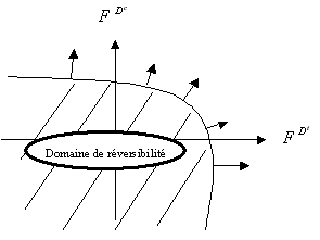
Figure 3.1-a
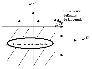
Figure 3.1-b
It is therefore decided to introduce a single criterion coupling the evolution of the two damage variables:
\(g({F}^{B},{F}^{d})=\sqrt{\alpha {\parallel {F}_{-}^{B}\parallel }^{2}+(1-\alpha ){({F}_{+}^{d})}^{2}}-K(\varepsilon )\le 0\) eq 3.1-1
where \(K(\varepsilon )\) is a threshold depending on the state of deformation (this point will be commented on in section [§ 3.2]).
The evolution of the damage variables is then determined by the Kuhn-Tucker conditions:
\(\{\begin{array}{cc}\begin{array}{}\dot{d}=0\\ \dot{B}=0\iff \dot{D}=0\end{array}& \text{pour}g<0\\ & \\ \begin{array}{}\dot{d}\ge 0\\ {\dot{B}}_{i}\le 0\iff {\dot{D}}_{i}\ge 0\end{array}& \text{pour}g=0\end{array}\) eq 3.1-2
Note:
The criterion only involves the positive part \({F}_{+}^{d}\) of \({F}^{d}\) and negative \({F}_{-}^{B}\) of \({F}^{B}\) in order to impose the growth of damage. This condition is ensured in the dissipation potential by the introduction of the indicator functions \({I}_{{ℝ}^{+}}(\dot{d})\) and \({I}_{{ℝ}^{-}}({\dot{B}}_{i})\) (equivalent to \({I}_{{ℝ}^{+}}({\dot{D}}_{i})\) ) .
Note:
The elliptical criterion is convex in the thermodynamic force space, which ensures the convexity of the dissipation potential.
In the context of generalized standard materials, the evolution of internal variables follows the flow law associated with the criterion via the principle of normality:
\(\dot{B}=\dot{\eta }\frac{\partial g}{\partial {F}^{B}}=\dot{\eta }\frac{\alpha {F}_{-}^{B}}{\sqrt{\alpha {\parallel {F}_{-}^{B}\parallel }^{2}+(1-\alpha ){({F}_{+}^{d})}^{2}}}\) eq 3.1-3
\(\dot{d}=\dot{\eta }\frac{\partial g}{\partial {F}^{d}}=\dot{\eta }\frac{(1-\alpha ){F}_{+}^{d}}{\sqrt{\alpha {\parallel {F}_{-}^{B}\parallel }^{2}+(1-\alpha ){({F}_{+}^{d})}^{2}}}\) eq 3.1-4
We can integrate the common denominator into the Lagrange multiplier to have a simpler relationship:
\(\dot{B}=\dot{\eta }\frac{\partial g}{\partial {F}^{B}}=\dot{\gamma }\alpha {F}_{-}^{B}\) eq 3.1-5
\(\dot{d}=\dot{\eta }\frac{\partial g}{\partial {F}^{d}}=\dot{\gamma }(1-\alpha ){F}_{+}^{d}\) eq 3.1-6
This system uses a single plastic multiplier \(\dot{\gamma }\).
The evolution equations ensure the positivity of the dissipation potential:
\({F}^{B}:\dot{B}+{F}^{d}\dot{d}=\dot{\mathrm{\gamma }}\left[\mathrm{\alpha }{\parallel {F}_{-}^{B}\parallel }^{2}+(1-\mathrm{\alpha }){({F}_{+}^{d})}^{2}\right]\ge 0\) eq 3.1-7
Note:
From a theoretical point of view, the compression damage and the eigenvalues of the tensile damage tensor can reach a value of 1. This corresponds to a completely damaged element whose stiffness is zero, as well as the stress. From a numerical point of view, this situation leads to instabilities since the stiffness matrix becomes singular. A programming choice is made to avoid this problem: limit the damage to a value \(1–\mathrm{tol}\) where \(\mathrm{tol}\) is set to 0.01. The need to limit damage in this way results in the appearance of residual stiffness. In other words, even if the material is completely damaged in one direction, it continues to resist, admittedly weakly, in that direction.
3.2. Deformation-dependent threshold function#
In order to better control the asymmetry of the behavior between tension and compression (ratio 10 of the rupture limits), we introduced a threshold function dependent on the state of deformation in the criterion [éq 3.1-1]. The role of this threshold function is to push back the elastic limit under compression. It is also desired that the breaking stress in simple tension cannot be exceeded during a biaxial test (cf. [bib1] for a detailed study of the threshold function).
The function we offer is as follows:
\(K(\varepsilon )={k}_{0}-{k}_{1}{(\text{tr}\varepsilon )}_{-}\text{arctan}(-\frac{{(\text{tr}\varepsilon )}_{-}}{{k}_{2}})\) eq 3.2-1
This threshold function introduces 3 parameters for the model.
Note:
This function has not been optimized for triaxial compression loads. In this respect, it should be noted that the law ENDO_ORTH_BETON was designed to describe tensile damage in a more detailed manner, the description of compression damage remaining isotropic. Another law of behavior must therefore be used for applications involving high triaxial compression loads.
When the deformation trace is positive, the threshold remains constant: \(K(\mathrm{\varepsilon })={k}_{0}\). The threshold increases when compression is applied, which makes it possible to push back the elastic limit, and therefore the breaking limit. Note that the « arctan » function was introduced to better represent the rupture envelope in the case of biaxial tests (a detailed study can be found in [bib1]).
The [Figure 3.2-a] shows us the comparison between the elastic limit provided by a constant threshold and that obtained with a threshold dependent on the trace of the deformations in the case of biaxial tests under plane stress.
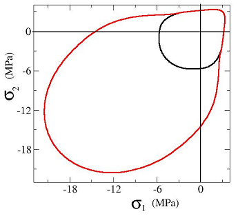
Figure 3.2-a: Envelope of the elasticity domain for biaxial loads in plane stress.