4. Parameter study#
In addition to classical elastic parameters \(E\) (Young’s modulus) and \(\nu\) (Poisson’s ratio), the model involves 6 additional parameters:
Code_Aster |
Function |
Dimension* |
Identification** |
|
\(\alpha\) |
|
Coupling Parameter |
Without |
1 |
\({k}_{0}\) |
K0 |
Constant part of the threshold |
\(\mathrm{MPa}\) |
2 |
\({k}_{1}\) |
K1 |
Threshold Parameter |
\(\mathrm{MPa}\) |
3 |
\({k}_{2}\) |
K2 |
Threshold Parameter |
Without |
3 |
\({\gamma }_{B}\) |
|
Blocked energy relating to traction |
\(\mathrm{MJ}/{m}^{3}=\mathrm{MPa}\) |
2 |
\({\gamma }_{d}\) |
|
Blocked energy related to compression |
\(\mathrm{MJ}/{m}^{3}=\mathrm{MPa}\) |
3 |
You multiply the parameters in MegaPascals (\(\mathrm{MPa}\)) by 106 if you work in Pascals (\(\mathrm{Pa}\)).
** Parameters should be calibrated in the following order:
we set the parameter \(\alpha\)
identification of \({k}_{0}\) and \({\gamma }_{B}\) on a simple tensile test
identification of \({k}_{1}\), \({k}_{2}\) and \({\gamma }_{d}\) on a simple compression test and a biaxial test (\({\mathrm{\sigma }}_{1}={\text{\beta \sigma }}_{2}\) with \(\beta =-\mathrm{0,2}\) to verify that the tensile breaking stress is not exceeded)
Let us now study the influence of the various parameters on the response of the model in a little more detail.
4.1. Influence of parameter \(\alpha\)#
The role of the parameter \(\alpha\) is to control the influence ratio of the two associated thermodynamic forces in the evolution criterion. A parameter \(\alpha\) close to \(1\) favors the evolution of tensile damage and a parameter \(\alpha\) close to \(0\) favors the evolution of compression damage. We decided to use a constant setting for reasons of simplicity.
If damage is caused by simple compression in direction 1, cracks are created in the planes orthogonal to \({\overrightarrow{e}}_{2}\) and \({\overrightarrow{e}}_{3}\). If you then pull in direction 2 or 3, you « see » these cracks. To achieve this effect in the model, compression must cause not only compression damage, but also tensile damage. On the other hand, if we start with traction in direction 1, the cracks in the plane perpendicular to \({\overrightarrow{e}}_{1}\) will not be very open (slight deformation at break), so we can think that we will not « see » them if we then compress in direction 2 or 3. It is concluded that it is necessary to take \(\alpha \ne 0\) and \(\alpha \ne 1\) to have a coupling, and close to 1 to promote the evolution of traction damage during compressions. There will also be a small evolution of compression damage during pull-ups, devoid of physical sense, but it will not be annoying if this damage remains low.
4.1.1. Uniaxial tests#
The aim here is to observe the influence of the parameter \(\alpha\) in the case of simple traction and simple compression. The other parameters of the model are taken constant for our series of tests:
\(E=28800\text{MPa},\nu =0.2,{k}_{0}={3.10}^{-4}\text{MPa},{k}_{1}=10\text{MPa},{k}_{2}={2.10}^{-4},{\gamma }_{B}=0{\text{MJ/m}}^{\mathrm{3,}}{\gamma }_{d}=0.06{\text{MJ/m}}^{3}\)
For compression, a significant difference in peak stress is observed (cf. [Figure 4.1.1-b]). The closer \(\alpha\) is to \(1\), the higher the threshold constraint. This phenomenon is accentuated when we take a threshold dependent on deformations as is the case on [Figure 4.1.1-b].
Note:
The fact that the threshold stress is more sensitive in compression than in tension is due to the fact that we take a value of \(\alpha\) close to \(1\) , preferring tensile damage. The effect would be reversed if one taken \(\alpha\) near \(0\) .
The parameter \(\alpha\) also influences the relative speed of damage evolution via the law of normality of the flow. The closer \(\alpha\) is to \(1\), the more rapidly the lateral tension damage \({D}_{\text{yy}}\) increases compared to the compression damage \(d\) as seen on the [Figure 4.1.1-c].
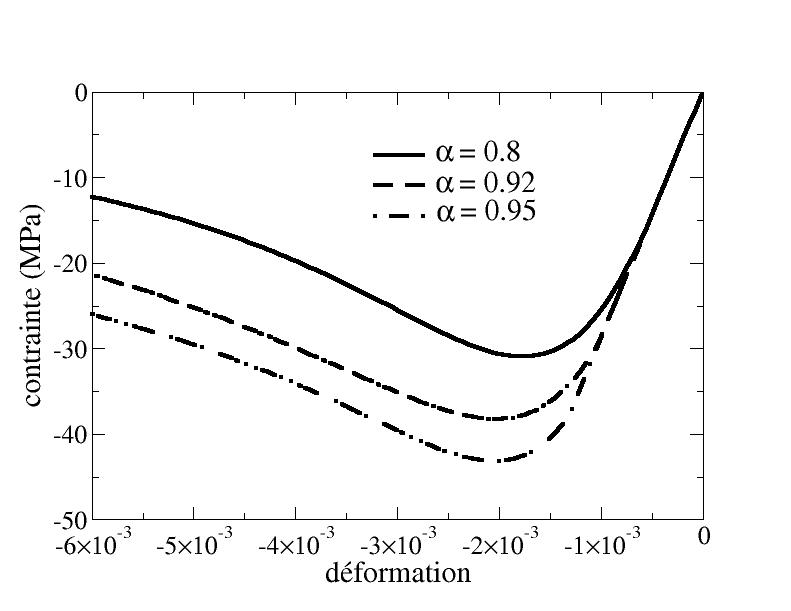
Figure 4.1.1-b: Influence of the parameter \(\alpha\) on simple compression
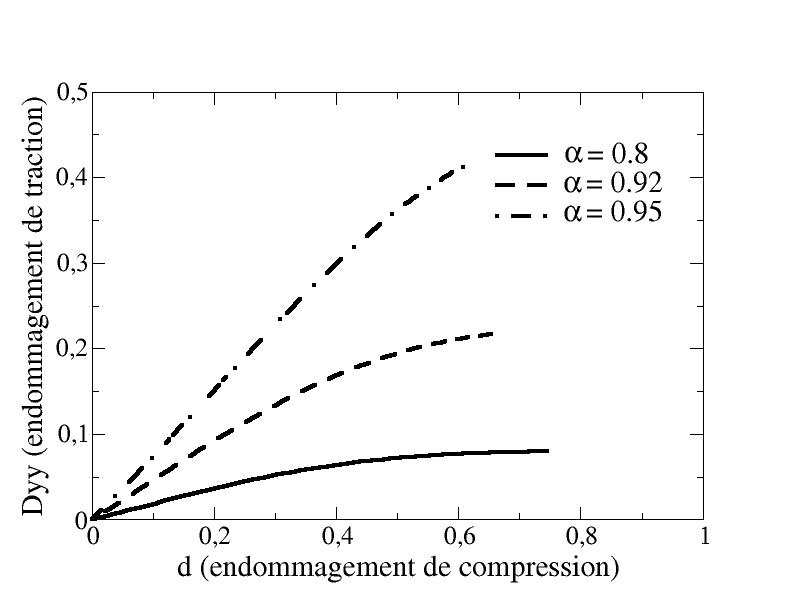
Figure 4.1.1-c: Evolution of tensile damage versus****compression damage for simple compression
4.1.2. Warning#
In a simple compression test, cracks are created orthogonally to the directions of positive deformation, and influence the subsequent tensile behavior. We introduced coupling in order to represent this phenomenon. However, it can be seen from the simple compression test that lateral tension damage does not reach ruin (\({D}_{\text{yy}}^{\text{lim}}<1\)) when compression damage \(d\) tends to \(1\). This is a limitation of the model.
However, it is possible to reach ruin for a value of \(\alpha\) closer to \(1\). Tensile damage will then evolve more quickly than compression damage (cf. [Figure 4.1.2-a]). Unfortunately the stress-strain response then causes a snap‑back to appear (cf. [Figure 4.1.2-b]) devoid of physical meaning, so that it is necessary to exclude these values from \(\alpha\).
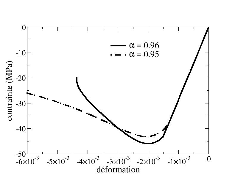
Figure 4.1.2-a: Effect of a parameter \(\alpha\) very close to 1 on the response stress-strain in simple compression
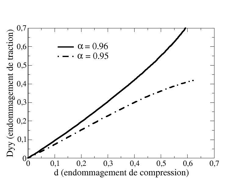
Figure 4.1.2-b: Effect of a parameter \(\alpha\) very close to 1 on the relative evolution of tensile and compression damage under simple compression
4.1.3. Identifying parameter \(\alpha\)#
There is a critical value for parameter \(\alpha\) clear of which we encounter the disadvantages set out in section [§ 4.1.2]. This critical value depends on the other parameters but we do not have an empirical formula to find it. It is therefore preferable to use a value of \(\alpha\) around \(\mathrm{0,9}\) which causes compression damage to develop more rapidly than tensile damage in the simple compression test, so that it is then impossible to observe tensile failure in the directions perpendicular to that of compression.
4.2. Influence of parameters \({\gamma }_{B}\) and \({\gamma }_{d}\)#
The introduction of blocked energy depending on the damage variables makes it possible to control the rate of evolution of the damage, and therefore makes it possible to control the shape of the stress-deformation curve.
4.2.1. Simple tensile test#
In the simple tensile test, only the part of the blocked energy relating to the tensile damage has a real influence. The stress-strain curve is shown on [Figure4.2.1-a] for various values of \({\gamma }_{B}\). We can see that the bigger \({\gamma }_{B}\), the greater the breaking stress, and the wider the peak. This is because the blocked energy slows the damage from progressing, as shown in [Figure4.2.1-b].
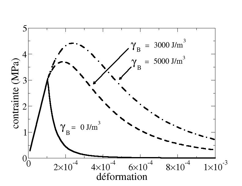
Figure 4.2.1-a: Influence of blocked energy on a simple tensile test
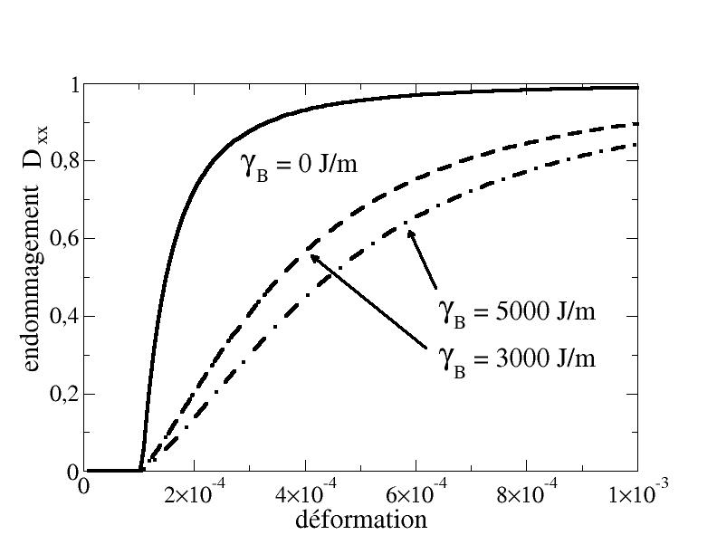
Figure 4.2.1-b: Influence of blocked energy on the rate of evolution of damage
4.2.2. Simple compression test#
In the simple compression test, only the part of the blocked energy relating to the compression damage has a real influence. However, the parameter \({\gamma }_{d}\) is less easy to calibrate because the criterion threshold depends on the deformation state. We will immediately explain this point in the next warning.
Note:
Theoretically, the warning that we are about to present is also valid in traction. In practice, we are not confronted with it because we always favor tensile damage by taking a coupling parameter \(\alpha\) close to 1, and we do not take a value of \({\gamma }_{d}\) that is too large (the behavior of concrete under tension is almost fragile) .
4.2.2.1. Warning#
The introduction of blocked energy should make it possible to slow down the evolution of compression damage, and therefore should make it possible to round the shape of the peak in a simple compression test. However, a warning must be expressed regarding the use of this blocked energy. The thermodynamic force that drives the evolution of compression damage is the sum of two terms: one corresponding to the derivation of elastic energy, dependent on deformation and damage, positive, and the other corresponding to the derivation of blocked energy, depending only on the damage, negative. However, when the damage increases, it is possible that the term corresponding to the blocked energy is too large in absolute value compared to that corresponding to the elastic energy, which can prevent the evolution of the damage.
\(\begin{array}{ccc}{F}^{d}={F}_{\mathrm{élastique}}^{d}(\varepsilon ,d)+{F}_{\mathrm{bloquée}}^{d}(d)& \text{avec}& \{\begin{array}{}{F}_{\mathrm{élastique}}^{d}(\varepsilon ,d)\ge 0\\ {F}_{\mathrm{bloquée}}^{d}(d)\le 0\end{array}\\ {F}_{\mathrm{élastique}}^{d}(\varepsilon ,d)+{F}_{\mathrm{bloquée}}^{d}(d)\le 0& \Rightarrow & d\text{n'évolue plus}\end{array}\)
This problem arises when considering a constant threshold in the criterion. In this case, the [Figure 4.2.2.1-a] shows us the influence of the introduction of blocked energy on the stress-strain curve in a simple compression test. It is observed that the introduction of this energy, by slowing down the evolution of compression damage, makes it possible at first to increase the height of the stress peak as well as the width of the peak. However, we note that a snap-back appears on the two curves where blocked energy has been added. This is due to the fact that the evolution of compression damage is slowed down but the tensile damage is not affected. This is illustrated on [Figure 4.2.2.1-b], which shows a stabilization of compression damage combined with a rapid increase in tensile damage.
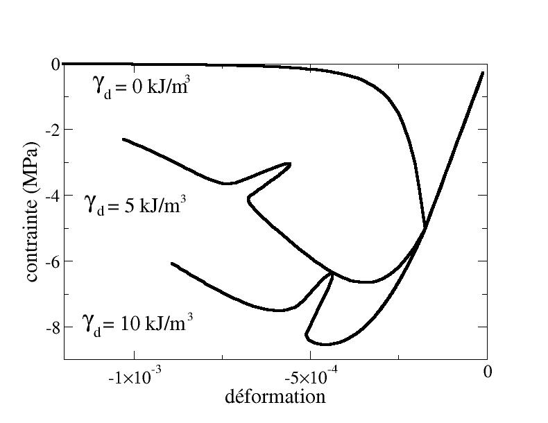
Figure 4.2.2.1-a: Influence of blocked energy in a simple compression test
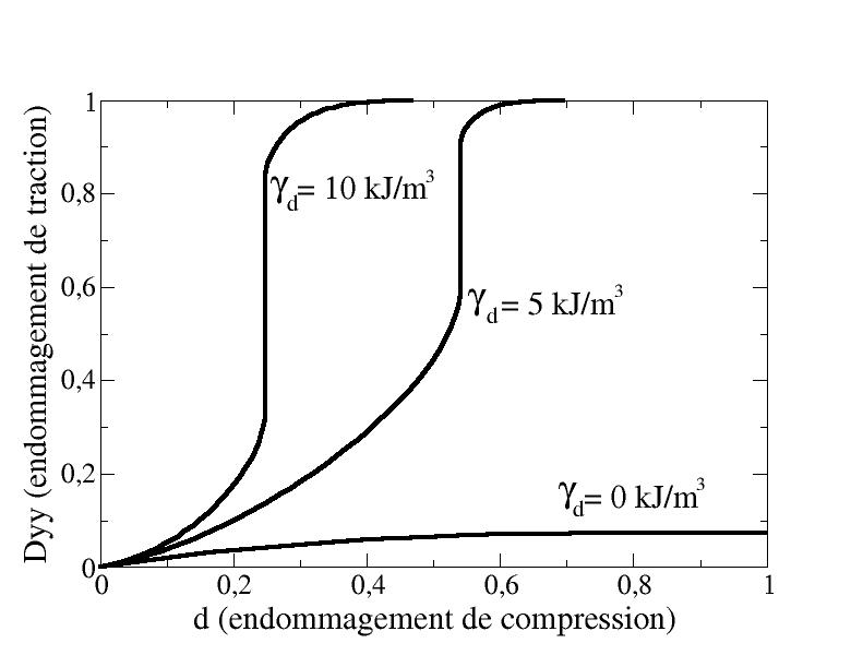
Figure 4.2.2.1-b: Evolution of lateral traction damage as a function of compression damage
4.2.2.2. Combination of blocked energy and deformation-dependent threshold#
When using a threshold dependent on the state of deformation, the force associated with the elastic energy remains greater than that associated with the blocked energy because, for the same state of damage, the criterion is reached for higher levels of deformation. In this case, we can see the influence of the introduction of blocked energy on the response of the model under compression. This makes it possible to control the shape of the peak (cf. [Figure 4.2.2.2-a]), that is to say the breaking stress as well as the deformation at break. We can also see on the [Figure 4.2.2.2-b] that the greater the parameter associated with the blocked energy, the more the lateral tension damage evolves compared to the compression damage. However, it is obvious that if we take a parameter \({\gamma }_{d}\) that is too big, we find the problems mentioned above.
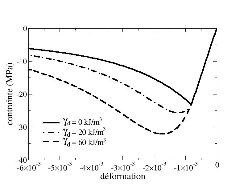
Figure 4 .2.2.2-a: Influence of blocked energy in a simple compression test
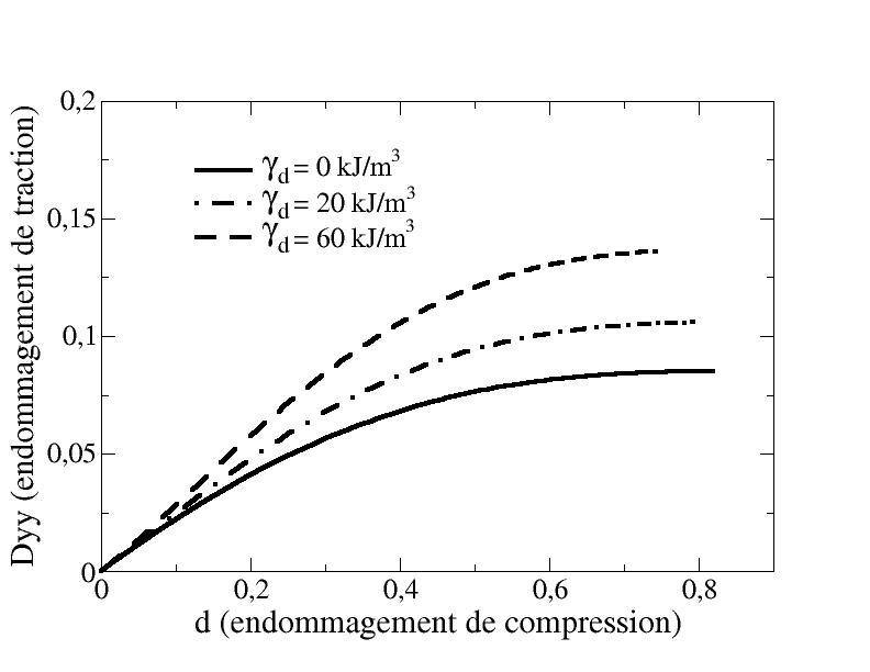
Figure 4 *.2.2.2-b: Evolution of lateral traction damage****as a function of compression damage*
4.2.3. Identifying parameters#
Parameter \({\gamma }_{B}\) is identified on the simple tensile test. It allows you to adjust the height and width of the peak for this test. It should be set at the same time as threshold parameter \({k}_{0}\).
Parameter \({\gamma }_{d}\) is identified on the simple compression test. It allows you to adjust the height and width of the peak for this test. It should be set at the same time as threshold settings \({k}_{1}\) and \({k}_{2}\).
4.3. Influence of threshold function parameters#
The threshold function that is used involves three parameters:
\(K(\varepsilon )={k}_{0}-{k}_{1}{(\text{tr}\varepsilon )}_{-}\text{arctan}(-\frac{{(\text{tr}\varepsilon )}_{-}}{{k}_{2}})\) eq 4.3-1
In the case of a simple pull, only the parameter \({k}_{0}\) intervenes. As soon as the trace of the deformations becomes negative, as is the case in simple compression, the three parameters come into play. Parameter \({k}_{0}\) must therefore be calibrated beforehand on a simple tensile test. Parameters \({k}_{1}\) and \({k}_{2}\) will then be calibrated on a simple compression test and a biaxial test, with \({k}_{0}\) fixed.
4.3.1. Simple traction: influence of parameter \({k}_{0}\)#
If we take a blocked energy that does not depend on the tensile damage (\({\gamma }_{B}=0\)), the value of the breaking stress is totally determined by the value of \({k}_{0}\), \(\alpha\), and the elastic parameters:
\({\sigma }_{\mathrm{rupture}}^{2}=\frac{{k}_{0}E}{\sqrt{\alpha +2(1-\alpha )\frac{{\nu }^{4}}{{1+\nu }^{2}}}}\) eq 4.3.1-1
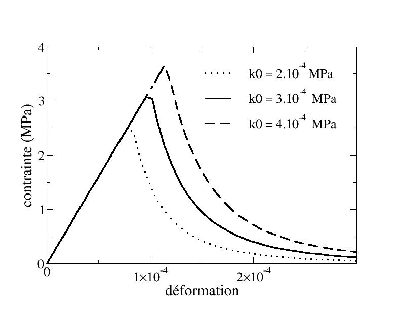
Figure 4.3.1-a: Dependence of the tensile breaking stres on the parameter \({k}_{0}\) ( \(E=32000\mathrm{Mpa}\) , \(\nu =0.2\) , ,, :math:`alpha =0.87`) **
Obviously, the greater \({k}_{0}\), the greater the tensile breaking stress as shown in [Figure 4.3.1-a].
Unfortunately, there is no analytic expression for breaking stress when \({\gamma }_{B}\ne 0\) is used. The dependence of the response on the parameter \({\gamma }_{B}\) is studied in paragraph [§ 4.2.1]. Parameters \({k}_{0}\) and \({\gamma }_{B}\) should be calibrated simultaneously.
4.3.2. Compression: influence of parameters \({k}_{1}\) and \({k}_{2}\)#
The role of the threshold function, which depends on the negative trace of the deformation, is to increase the compression fracture limit, in order to better control the asymmetry of concrete behavior between traction and compression.
In addition, we made the choice to take a threshold function to describe the fracture envelope of concrete in the case of biaxial loads. This choice was made for two reasons:
For these tests, we have experimental results (cf. [bib5]). Of course, these tests only concern the concrete used by [bib5], but they have common features that can seem to be generalized.
This makes it possible to expand the range of use of the model. Uniaxial tests are in fact insufficient to ensure the relevance of the model in the case of 3D calculations.
Note:
The model should not be used in the case of strong triaxial compressions, as the free energy and the threshold function have not been established to treat this case. It should be noted that the main objective of the model is to describe tensile damage in concrete.
4.3.2.1. Role of parameter \({k}_{1}\)#
Parameter \({k}_{1}\) is the parameter that allows you to increase the compression break limit. The [Figure 4.3.2.1-a].
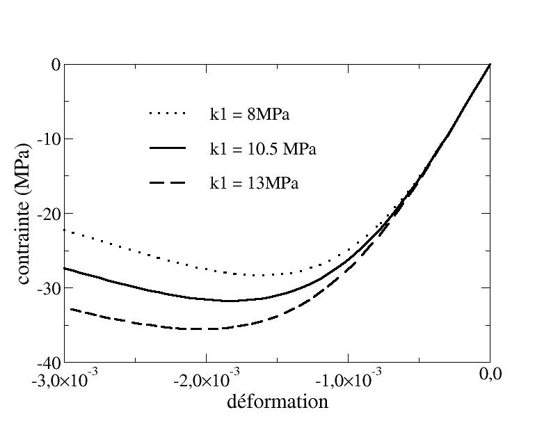
Figure 4.3.2.1-a: Dependence of the simple compression response on \({k}_{1}\) ( \(E=32000\mathrm{MPa},\nu =0.2,{k}_{0}={3.10}^{-4}\mathrm{MPa},{k}_{2}={6.10}^{-4},{\gamma }_{d}={6.10}^{-2}\mathrm{MJ}/{m}^{3}\)
4.3.2.2. Role of parameter \({k}_{2}\)#
To understand the role of the \({k}_{2}\) parameter, let’s go back to the path that led us to choose the threshold function [éq 3.2-1].
The first threshold function that has been tested is the linear function:
\(K(\varepsilon )={k}_{0}-{k}_{1}{(\text{tr}\varepsilon )}_{-}\) eq 4.3.2.2-1
This function makes it possible to increase the breaking stress in simple compression, but it poses a problem when interested in biaxial tests. The [Figure 4.3.2.2-a] shows us the envelope of the elastic domain for biaxial tests.
Note:
The envelope of the elasticity domain is different from the rupture envelope (for which we have experimental results). We study the envelope of the elasticity domain because it can be calculated analytically, unlike the rupture envelope, and because it is from this envelope that we have chosen our threshold function. However, the user must properly calibrate his parameters on the break envelope.
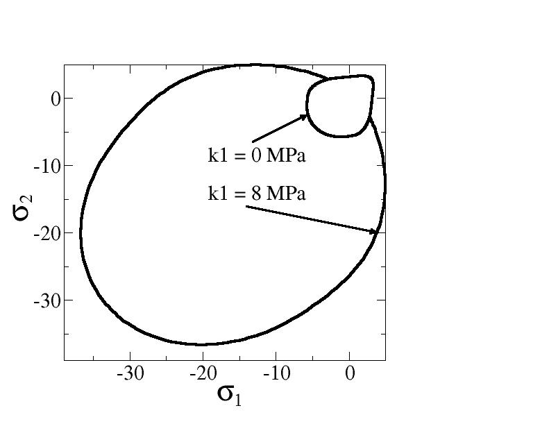
Figure 4.3.2.2-a: Elasticity domain envelope for biaxial tests with a linear threshold function
The linear variation of the threshold with deformation does not seem to be appropriate since swelling appears in zone \(({\mathrm{\sigma }}_{1}>\mathrm{0,}{\mathrm{\sigma }}_{2}<0)\) which gives excessively high tensile stress limits.
So we modified the threshold function:
\(K(\mathrm{\varepsilon })={k}_{0}-{k}_{1}{(\text{tr}\mathrm{\varepsilon })}_{-}\text{arctan}(-\frac{{(\text{tr}\mathrm{\varepsilon })}_{-}}{{k}_{2}})\) eq 4.3.2.2-2
The fact that the arctan function has a level makes it possible to find a linear threshold when the trace of the deformations increases in absolute value. The fact that it is zero at the origin makes it possible to slow down the increase in the threshold near this origin.
We can see on the [Figure 4.3.2.2-b] the effect of the introduction of the new threshold function with respect to the linear function on the elasticity domain for the same value of the parameter \({k}_{1}\). This new threshold function makes it possible to avoid the swelling phenomenon observed with the linear function when the value of the parameter \({k}_{2}\) is increased (the case \({k}_{2}=0\) corresponds to the linear function). The other effect of the parameter \({k}_{2}\) is to reduce the stress to initiate the damage, which implies a decrease in the breaking stress (the opposite effect of \({k}_{1}\)) as shown in [Figure 4.3.2.2-c].
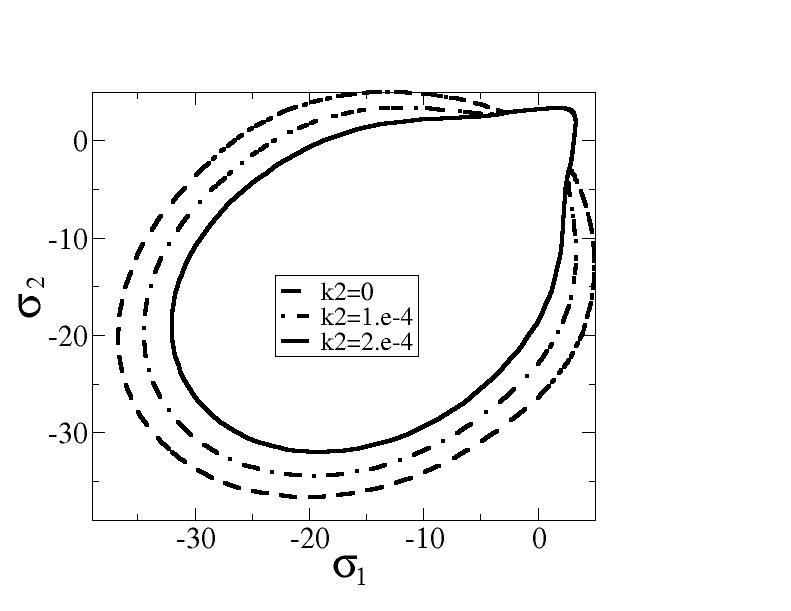
Figure 4.3.2.2-b: Elasticity domain with the two-parameter threshold function
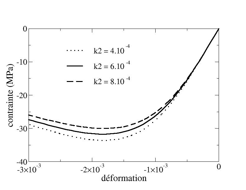
Figure 4.3.2.2-c: Dependence of the response in simple compression on \({k}_{2}\) ( \(E=32000\text{MPa},\nu =0.2,{k}_{0}={3.10}^{-4}\text{MPa},{k}_{1}=10.5\text{MPa},{\gamma }_{d}={6.10}^{-2}{\text{MJ/m}}^{3}\) )
4.3.3. Identifying parameters#
Parameters \({\gamma }_{d}\), \({k}_{1}\), and \({k}_{2}\) are identified simultaneously. The parameters \({k}_{1}\) and \({\gamma }_{d}\) make it possible to adjust the breaking stress in simple compression and the parameter makes it possible to avoid the « swelling » of the elastic domain envelope (and therefore of the rupture envelope) for biaxial tests. The bigger \({k}_{1}\) you take, the bigger \({k}_{2}\) should be.
4.4. Report on the study of parameters#
Despite the relative simplicity of the model, and the low number of parameters to be identified (6), the number of experimental data available to the engineer is often, if not always, less than the number of parameters to be identified. This only implies the arbitrariness of the choice of certain parameters. In summary, here is the order in which the parameters should be chosen:
For the \(\alpha\) parameter, a value between \(\mathrm{0,85}\) and \(\mathrm{0,9}\) is recommended.
Parameters \({k}_{0}\) and \({\gamma }_{B}\) must be identified simultaneously on a simple tensile test (no analytical formula in case \({\gamma }_{B}\ne 0\)).
Parameters \({\gamma }_{d}\), \({k}_{1}\), and \({k}_{2}\) must be identified simultaneously. The easiest way is to set the parameter \({k}_{2}\) to \({6.10}^{-4}\) (value for which it is probable that no swelling of the rupture envelope is observed (cf. [§ 4.3.2.2]) for biaxial tests), and to calibrate \({\gamma }_{d}\) and \({k}_{1}\) on a simple compression test. We then check if the break envelope is correct, we modify \({k}_{2}\) if necessary and we start again for \({\gamma }_{d}\) and \({k}_{1}\).
Examples of parameter sets can be found in section 6 (validation on experimental tests). In addition, the test cases for identifying the parameters can be found in document [V6.04.176].