2. The MUMPS package#

2.1. History#

Package MUMPS implements a « massively » parallel multifrontend (”MUltifrontal Massively Parallel Sparse Direct Solver” [Mum]) developed during the European Project PARASOL (1996-1999) by the teams of three laboratories: CERFACS, ENSEEIHT - IRIT and RAL (I.S.Duff, P.R.Amestoy, J.Koster and J.Y.L’Excellent…) by the teams of three laboratories:, - and (I.S.Duff, P.R.Amestoy, J.Koster and J.Y.L’Excellent…).

Since this finalized version (MUMPS 4.04 22/09/99) and public (royalty-free), forty other versions have been delivered. These developments correct anomalies, extend the scope of use, improve ergonomics and above all, enrich functionalities. MUMPS is therefore a sustainable product, developed and maintained by a dozen people belonging to academic entities divided between Bordeaux, Lyon and Toulouse: IRIT, CNRS, CERFACS, INRIA/ENS Lyon and University of Bordeaux I.

_images/10000200000001340000006F10AD0E2581A6A5F2.png

_images/1000020000000048000000484C7511A7EE658C2A.png

Figure 2.1-1._ Logos of the main contributors to MUMPS [Mum].

The product is public and can be downloaded from its website: http://graal.ens-lyon.fr/MUMPS. There are around 1000 direct users (including 1/3 Europe + 1/3 USA) not including those who use it via the libraries that reference it: PETSc, TRILINOS, Matlab and Scilab… Its site offers documentation (theoretical and user), links, application examples, as well as a discussion forum (in English) outlining the feedback on the product (bugs, installation problems, advice…).

Each year, a dozen algorithmic/computer works lead to improvements to the package (thesis, post-doc, research work, etc.). On the other hand it is used regularly for industrial studies (EADS, CEA, BOEING,, GéoSciences Azur, SAMTECH, Code_Aster…).

Figure 2.1-2._ The home page of the MUMPS [Mum] website.

Since 2015, a consortium between academic teams, industrial teams and software publishers has been set up around the product: the MUMPS [MUC] consortium. It should make it possible to better ensure its development, distribution and sustainability.

It was managed by the INRIA and brought together at the end of 2015: EDF, ALTAIR, MICHELIN,, LSTC,, SIEMENS, ESI, TOTAL (members) and CERFACS, INPT,, BELOVA (members) and the University of Bordeaux (members) at the end of 2015:,,,,,,,,,, INRIA ENS founders).

Figure 2.1-3._ The home page of the website dedicated to the consortium [MUC].

2.2. Main characteristics#

MUMPS implements a multifront [ADE00] [] [ADKE01] [AGES06] performing a factorization \(LU\) or \(LD{L}^{T}\) (cf. §1.4). Its main characteristics are:

Wide scope of use: SPD, any symmetric, non-symmetric, non-symmetric, real/complex, simple/double precision, regular/singular matrix (all this scope is used in Code_Aster);

Admits**three methods of data distribution*: by element, centralized or distributed (the last two modes are used in*Code_Aster*);

Interfacing in Fortran (exploited), C, matlab and scilab.
Default setting and the possibility of letting the package choose some of its options depending on the type of problem, its nature and the number of processors (exploited).
Modularity (3 distinct interchangeable phases cf. §1.5 and figure 2.2.1) and opening some numerical arcana of MUMPS. The (very) advanced user can thus remove the result of certain pretreatments (scaling, pivoting, renumbering) from the product, modify them or replace them with others and reinsert them into the calculation chain specific to the tool;

Different**resolution strategies *: multiple second members, simultaneous resolutions and Schur complements (only the first two are used);

Different embedded or external**renumbers*: (PAR) METIS,, AMD, QAMD, AMF, PORD, (PT) SCOTCH, “provided by the user” (operated except the last one);

Related features: detection of small pivots/rank calculation (exploited), calculation of cores (soon to be exploited), error analysis and improvement of the solution (exploited), calculation of the inertia criterion for the Sturm test in modal calculation (exploited), low-rank compression (exploited), low-rank compression (exploited); use of the hollow character of the second member and simultaneous resolution of several linear systems (not exploited), calculation of a few terms of the opposite (not exploited), restart procedure (not yet exploited), manipulation of long integers (not yet exploited)?
Pre and post-processing: scaling, row/column permutation and 2x2 scale/block, iterative refinement (exploited);
Parallelism: potentially at 2 levels (MPI +OpenMP), asynchronous management of task/data flows and their dynamic reordering, compution/communication recovery; Data distribution associated with task distribution; This parallelism only starts at the level of the factorization phase, unless one of the parallel renumbers (PARMETIS or PTSCOTCH) has been chosen.
Memory: unloading factorized data to disk or not (In-Core or Out-Of-Core modes) with prior estimation of RAM consumption per processor in both cases (exploited).

*Figure 2.2-1._ Functional flowchart of MUMPS:**its three stages in parallel centralized/distributed and IC/ OOC. *

Note:

*In terms of parallelism, MUMPS uses two levels (cf. [R6.01.03]*§2.6.1): one external linked to the concurrent elimination of fronts (via MPI), the other internal, within each front (via BLAS « threads » or around low-rank compression algorithms) . *

Code_Aster’s native multifrontend method only uses the second level and in shared-memory parallelism (via OpenMP). So without overlay, dynamic reordering and data distribution between processors. On the other hand, through its fine connections with Code_Aster, it uses all the facilities of the memory manager JEVEUX (OOC, restart, diagnosis…) and the specificities of code modeling (structural elements, Lagranges) .

2.3. Let’s zoom in on a few technical points#

2.3.1. Swivel#

The pivoting technique consists in choosing a suitable term \({\tilde{A}}_{k}(k,k)\) (in the formula 1.4-3) to avoid dividing by a term that is too small (which would amplify the spread of rounding errors when calculating the following \({\tilde{A}}_{k+1}(i,j)\) terms). To do this, we switch rows (partial rotation) and/or columns (resp. total) to find the suitable denominator of (1.4-3). For example, in the case of a partial pivot, we choose as « pivot » the term \({\tilde{A}}_{k}(r,k)\) such as

\({\tilde{\mathrm{A}}}_{k}(r,k)\mathrm{\ge }u\underset{i}{\text{max}}\mathrm{\mid }{\tilde{\mathrm{A}}}_{k}(i,k)\mathrm{\mid }\text{avec}u\mathrm{\in }\mathrm{]}\mathrm{0,1}\mathrm{]}\) (2.3-1)

Figure 2.3-1._ Choosing the partial pivot at step k.

Hence an amplification of rounding errors to a maximum of (\(1+\)) at this stage. What’s important here is not so much to choose the largest term possible in absolute value (u =1) as to avoid choosing the smallest! The inverse of these pivots also occurs during the descend-ascent phase, so it is necessary to take care of these two sources of error amplification by choosing a median u. MUMPS, like many packages, offers by default u =0.01 (parameter MUMPSCNTL (1)).

To rotate, scalar diagonal terms are generally used, but also term blocks (2x2 diagonal blocks).

In MUMPS, two types of pivoting are implemented, one called “static” (during the analysis phase), the other called “numerical” (resp. numerical factorization). They can be configured and activated separately (cf. parameters MUMPS CNTL (1), CNTL (4) and ICNTL (6)). For matrices SPD or matrices with a dominant diagonal, these pivoting abilities can be deactivated without risk (the calculation will become faster), on the other hand, in other cases, they must be initialized to manage possible very small or zero pivots. This generally implies an additional filling of the factored one but increases numerical stability.

Notes:

This pivoting feature makes MUMPS essential for dealing with certain Code_Aster models (almost incompressible elements, mixed formulations, X- FEM…). At least until other direct solvers that include pivoting are available in the code.
The Aster user does not have direct access to the fine settings of these pivoting abilities. They are activated with the values by default. He can just unplug them partially by asking SOLVEUR/PRETRAITEMENTS =” SANS “(default=” AUTO”) .
The additional filling due to numerical pivoting must be scheduled as soon as possible in MUMPS (from the analysis phase). This is done by arbitrarily forecasting a percentage of memory overconsumption compared to the expected profile. This figure must be entered in percentages in the parameter MUMPS ICNTL (14) (accessible to the Aster user via the keyword SOLVEUR/PCENT_PIVOT initialized by default to 20%) . Subsequently, if this evaluation proves insufficient, depending on the type of memory management chosen (keyword SOLVEUR/GESTION_MEMOIRE), either the calculation stops at ERREUR_FATALE, or we Try a numerical factorization several times, each time doubling the size of this space reserved for pivoting.
Some products restrict their perimeter/robustness by not offering a pivoting strategy (SPRSBLKKT, MULT_FRONT_Aster…), others are limited to scalar pivots (CHOLMOD, PastiX, TAUCS, WSMP…) or propose specific strategies (disturbance method+Bunch-Kaufmann correction for PARDISO, Bunch-Parlett for SPOOLES…) or propose specific strategies (disturbance method+Bunch-Kaufmann correction for, Bunch-Parlett for…) .

2.3.3. Reliability of calculations#

To estimate the quality of the solution of a linear system [ADD89] [Hig02], MUMPS proposes numerical tools deduced from the theory of the inverse analysis of rounding errors initiated by Wilkinson (1960). In this theory, rounding errors due to several factors (truncation, finite arithmetic operation, etc.) are assimilated to disturbances on the initial data. This makes it possible to compare them to other sources of error (measurement, discretization…) and to manipulate them more easily via three indicators obtained in post-processing:

Conditioning \(\mathrm{cond}(K,f)\): it measures the sensitivity of the problem to the data (unstable, poorly formulated/discretized problem…). That is to say, the multiplying factor that the manipulation of the data will affect the result. To improve it, we can try to change the formulation of the problem or to balance the terms of the matrix, outside of MUMPS or via MUMPS (SOLVEUR/PRETRAITEMENTS =” OUI “in Code_Aster).
The reverse error \(\mathrm{be}(K,f)\) (“backward error”): it measures the propensity of the resolution algorithm to transmit/amplify rounding errors. A tool is said to be « reliable » when this figure is close to machine precision. To improve it, you can try to change the resolution algorithm or to modify one or more of its steps (in Code_Aster you can play on the parameters SOLVEUR/TYPE_RESOL, PRETRAITEMENTS and RENUM).
The direct error \(\mathrm{fe}(K,f)\) (“forward error”): it is the product of the previous two figures and provides a increase in the relative error on the solution.

\(\frac{\parallel \delta \text{u}\parallel }{\parallel u\parallel }<\underset{\text{fe}(K,f)}{\underset{\underbrace{}}{\text{cond}(K,f)\times \text{be}(K,f)}}\) (2.3-4)

We can give a graphical representation (cf. figure 2.3-2) of these notions by expressing the inverse error as the difference between « the initial data and the disturbed data », while the direct error measures the difference between « the exact solution and the solution actually obtained » (that of the problem disturbed by rounding errors).

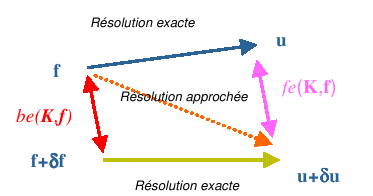
Figure 2.3-2._ Graphic representation of the concept of forward and reverse errors.

In the context of linear systems, the inverse error is measured via the balanced residual

\(\text{be}(K,f):=\underset{j\in J}{\text{max}}\frac{{\mid f-\text{Ku}\mid }_{j}}{{(\mid K\mid \mid u\mid +\mid f\mid )}_{j}}\) (2.3-5)

You can’t always assess it on every index (\(J\ne {\left[\mathrm{1,}N\right]}_{{\rm N}}\)). In particular when the denominator is very small (and the numerator is not zero), we prefer the formulation (with \({J}^{\text{*}}\) such as \(J\cup {J}^{\text{*}}={\left[\mathrm{1,}N\right]}_{{\rm N}}\))

\({\text{be}}^{\text{*}}(\mathrm{K},\mathrm{f})\mathrm{:}\mathrm{=}\underset{j\mathrm{\in }{J}^{\text{*}}}{\text{max}}\frac{{\mathrm{\mid }\mathrm{f}\mathrm{-}\text{Ku}\mathrm{\mid }}_{j}}{{(\mathrm{\mid }\mathrm{K}\mathrm{\mid }\mathrm{\mid }\mathrm{u}\mathrm{\mid })}_{j}+{\mathrm{\parallel }{\mathrm{K}}_{j\text{.}}\mathrm{\parallel }}_{\mathrm{\infty }}{\mathrm{\parallel }\mathrm{u}\mathrm{\parallel }}_{\mathrm{\infty }}}\) (2.3-6)

where \({K}_{j}\) . represents the \({j}^{\mathrm{ième}}\) row of the \(K\) matrix. To these two indicators, we associate two estimates of matrix conditioning (one linked to the lines selected in set \(J\) and the other to its complementary \({J}^{\text{*}}\)): \(\mathrm{cond}(K,f)\) and \({\mathrm{cond}}^{\text{*}}(K,f)\). The theory then provides us with the following results:

The approximate solution u is the exact solution of the disturbed problem

\(\begin{array}{c}(\mathrm{K}+\delta \mathrm{K})\mathrm{u}\mathrm{=}(\mathrm{f}+\delta \mathrm{f})\\ \text{avec}\delta {\mathrm{K}}_{\text{ij}}\mathrm{\le }\text{max}(\text{be},{\text{be}}^{\text{*}})\mathrm{\mid }{\mathrm{K}}_{\text{ij}}\mathrm{\mid }\\ \text{et}\delta {\mathrm{f}}_{i}\mathrm{\le }\text{max}(\text{be}\text{.}\mathrm{\mid }{\mathrm{f}}_{i}\mathrm{\mid },{\text{be}}^{\text{*}}\text{.}{\mathrm{\parallel }{\mathrm{K}}_{i\text{.}}\mathrm{\parallel }}_{\mathrm{\infty }}{\mathrm{\parallel }\mathrm{u}\mathrm{\parallel }}_{\mathrm{\infty }})\end{array}\) (2.3-7)

We have the following increase (*via*the direct error :math:`mathrm{fe}(K,f)`) on**the relative error in solution*

\(\frac{\parallel \delta \text{u}\parallel }{\parallel u\parallel }<\underset{\text{fe}(K,f)}{\underset{\underbrace{}}{\text{cond}\times \text{be}+{\text{cond}}^{\text{*}}\times {\text{be}}^{\text{*}}}}\) (2.3-8)

In practice, we mainly look at this last estimate \(\mathrm{fe}(K,f)\) and its components. Its order of magnitude indicates roughly the number of « true » decimals of the solution calculated. For poorly conditioned problems, a tolerance of \({10}^{\text{-3}}\) is not uncommon, but it should be taken seriously because this type of pathology can seriously disrupt a stone.

Even within the very precise framework of solving linear systems, there are many ways to define the sensitivity to rounding errors of the problem in question (i.e. its conditioning). The one selected by MUMPS and, which is a reference in the field (cf. Arioli, Demmel and Duff 1989), is inseparable from the “backward error” of the problem. The definition of one does not make sense without defining the other. This type of conditioning should therefore not be confused with the concept of classical matrix conditioning.

On the other hand, the packaging provided by step MUMPS takes into account the SECOND MEMBRE of the system as well as the CARACTERE CREUX of the matrix. Indeed, it is not worth taking into account possible rounding errors on zero matrix terms and therefore not provided to the solver! The corresponding degrees of freedom do not « speak to each other » (seen from the finite element lens). Thus, this MUMPS conditioning respects the physics of the discretized problem. It does not plunge the problem back into the too rich space of full matrices.

Thus, the conditioning figure displayed by MUMPS is much less pessimistic than the standard calculation that another product can provide (Matlab, Python…). But let’s not forget that it is only his product with the “backward error”, called “forward error”, that is of interest. And only, as part of a linear system resolution*via* MUMPS.

Notes:

This solution quality analysis is not limited to linear solvers. It is also available, for example, for modal solvers [Hig02].
In MUMPS, the estimators \(\mathrm{fe},\mathrm{be},{\mathrm{be}}^{\text{*}}`*, *:math:\)mathrm{cond}`*, and*:math:{mathrm{cond}}^{text{*}} are accessible via, respectively, the variables RINFO (9/7/8/10 and 11). These post-treatments are a bit expensive (~ up to 10% of the calculation time) and therefore deactivable (via* ICNTL (11)) .
For the Code_Aster user these MUMPS parameters are not directly accessible. They are displayed in a specific box in the message file (labeled « monitoring MUMPS ») if you enter the keyword INFO =2 in the operator. On the other hand, this feature is only activated if he chooses to estimate and test the quality of his solution via the parameter SOLVEUR/RESI_RELA. Depending on the Aster operators, this parameter is by default unplugged (negative value) or set to 10-6. When activated (positive value), we test whether the direct error \(\mathit{fe}(\mathrm{K},\mathrm{f})\) * is much less than RESI_RELA. If this is not the case, the calculation stops in ERREUR_FATALE by specifying the nature of the problem and the offending values.
Activating this feature is not essential (but often useful) when the solution sought is itself corrected by another algorithmic process (Newton algorithm, Newmark diagram): in short, in linear operators * THER_LINEAIRE, MECA_STATIQUE, STAT_NON_LINE, DYNA_NON_LINE…
This type of functionality seems not very present in libraries: LAPACK, Nag, HSL…

2.3.4. Memory Management (In-Core versus Out-Of-Core)#

We have seen that the major drawback (cf. §1.7) of direct methods lies in the size of the factored method. To allow larger systems to be moved to RAM, MUMPS suggests unloading this object onto disk: this is the Out-Of-Core mode (keyword GESTION_MEMOIRE =” OUT_OF_CORE “) as opposed to the In-Core mode (keyword GESTION_MEMOIRE =” IN_CORE”) where all data structures reside in RAM (cf. figures 2.2-1 and 2.3-3). This RAM economy mode is complementary to the data distribution that parallelism naturally induces. The added value of OOC is therefore especially significant for moderate numbers of processors (<32 processors).

On the other hand, the MUMPS team was very attentive to the additional CPU cost generated by this practice. By reworking the manipulations of the unloaded entities in the code algorithm, they were able to limit these additional costs to a strict minimum (a few percent and especially in the resolution phase).

Figure 2.3-3._ Two standard memory management types: entirely in RAM ( “IN_CORE” ) and RAM /disk (” OUT_OF_CORE “) .

These two memory management modes are « wireless ». No correction will be made later in the event of a problem. If you don’t know a priori you don’t know which of these two modes to choose and if you want to limit, as much as possible, the problems due to memory space defects, you can choose the automatic mode: GESTION_MEMOIRE =” AUTO “. Heuristics internal to Code_Aster then manage the memory contingencies of MUMPS by themselves according to the computer configuration (machine, parallelism) and the numerical difficulties of the problem.

In the same vein, an option with the same keyword, GESTION_MEMOIRE =” EVAL “, makes it possible to calibrate the needs of a calculation by displaying in the message file the memory resources required by the Code_Aster + MUMPS calculation.

Linear system size: 500000
Minimum RAM memory consumed by Code_Aster: 200 MB
Mumps memory estimation with GESTION_MEMOIRE =” IN_CORE “:3500 MB
Mumps memory estimate with GESTION_MEMOIRE =” OUT_OF_CORE “: 500 MB
Estimated disk space for Mumps with GESTION_MEMOIRE =” OUT_OF_CORE “:2000 MB

===> For this calculation, you therefore need a minimum quantity of memory RAM of

3500 MB if GESTION_MEMOIRE =” IN_CORE “,
500 MB if GESTION_MEMOIRE =” OUT_OF_CORE “.

When in doubt, use GESTION_MEMOIRE =” AUTO “.

Figure 2.3-4. _Message file snippet with GESTION_MEMOIRE =” EVAL “ .

Notes:

Parameters MUMPS * ICNTL (22)/ICNTL (23) allow you to manage these memory options. The user Aster activates them indirectly via the keyword SOLVEUR/GESTION_MEMOIRE.
Offloading to disk is entirely controlled by MUMPS (number of files, unloading/reloading frequency…). We just enter the memory location: it is quite naturally the working directory of the Aster executable specific to each processor (% OOC_TMPDIR =”. “).”). These files are automatically deleted by MUMPS when the associated MUMPS instance is destroyed. This therefore avoids disk congestion when different systems are factored into the same resolution.
Other OOC strategies would be possible or are already coded in some packages (PastiX, Oblio, TAUCS…). In particular, we think of being able to modulate the perimeter of the unloaded objects (cf. analysis phase that is sometimes expensive in RAM) and of being able to reuse them on disk during another execution (cf. POURSUITEau meaning Aster or partial factorization) .

2.3.5. Management of singular matrices#

One of the big strengths of the product is its management of singularities. It is not only able to detect numerical singularities [23] _ of a matrix and to synthesize the information for external use (ranking calculation, warning to the user, display of expertise…), but in addition, despite this difficulty, it calculates a regular « solution [24] _ « or even all or part of the associated kernel.

These new developments were one of the deliverables of ANR SOLSTICE [SOL]. We asked for them from the MUMPS team (in partnership with the Algo team from CERFACS) to make this product iso-functional compared to the other direct solvers of*Code_Aster*.

And in practice, how does MUMPS do it?

Broadly, when constructing the factored matrix, it detects rows with pivots [25] _ very small (compared to a criterion CNTL (3) [26] _ ). It lists them in the vector PIVNUL_LIST (1: INFOG (28)) and, depending on the case, it either replaces them with a pre-fixed value (via CNTL (5) [27] _ ), or it stores them separately. The block thus constituted (smaller in size) will subsequently be subjected to a QR*ad hoc* algorithm.

And lastly, iterative refinement iterations complete this conundrum. Since they only use this factorized « retouched » only as a preconditioner, and since they benefit, on the other hand, from the exact information of the matrix-vector product, they bring back [28] _ the « biased » solution in the right direction!

Notes:

Settings MUMPS ICNTL (13)/ICNTL (13)/(24)/ICNTL (25) and CNTL (3)/CNTL (5) enable these features to be activated. They cannot be changed by the user. As a matter of caution, we keep the feature activated at all times.
This feature can also be useful in modal calculation (filtering rigid modes) .

2.3.6. “Block Low-Rank” compression (BLR)#

This compression technique aims to facilitate large studies by reducing their time and memory costs. It is complementary to parallelism and to the algorithmic/functional pano of the product *. Its scope of use is almost complete.* We don’t have to choose between parallelism, this or that numerical refinement and these BLR compressions! All these features are compatible and their earnings often add up [29] _ .

Like the mp3, zip or pdf formats of our domestic and office uses, these compressions make it possible to reduce, with few losses, the expensive steps of MUMPS [30] _ . And this approximation generally does not disturb the precision and behavior of the encompassing mechanical calculations.

However, it is only interesting for large problems (N at least > 2.106ddls). Because these compressions involve an additional cost, it is necessary to compress only data blocks that are large enough and therefore likely to quickly compensate for this additional cost.

The gains observed on some Code_Aster studies vary from 20% to 80% (cf. figures 7.3-5/7.3-6). They increase with the size of the problem and its massive nature.

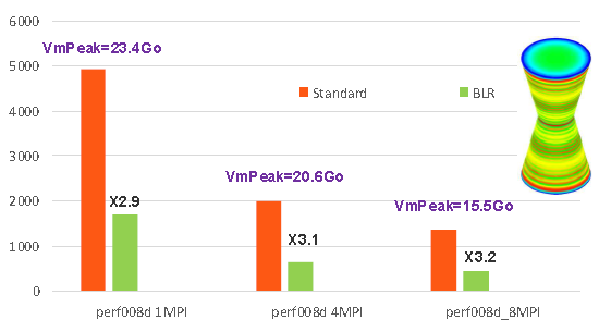
Figure 7.3-5: Example of gains provided by low-rank compressions on the perf008d performance test case (parameters by default, memory management in OOC, N=2M, NNZ =80M, =80M, Facto_ METIS4 =80M, Facto_ =7495M, conditioning=10 7*). As a function of the number of MPI processes activated, we plot the elapsed times consumed by the entire linear system resolution step in Code_Aster v13.1, its memory peak RAM, as well as the acceleration factor provided by BLR.*

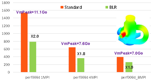
Figure 7.3-6: Example of gains provided by low-rank compressions on the perf009d performance test case (parameters by default, memory management in OOC, N=5.4M, NNZ =209M, =209M, Facto_ METIS4 =209M, Facto_ =5247M, conditioning=10 8*). As a function of the number of MPI processes activated, we plot the elapsed times consumed by the entire linear system resolution step in Code_Aster v13.1, its memory peak RAM, as well as the acceleration factor provided by BLR.*

Broadly, this strategy seeks to compress the large blocks of data most manipulated by the MUMPS multifront end: the big dense blocks of its elimination tree. This technique is based on the hypothesis (often verified empirically) that it is possible to renumber [31] _ the variables within these dense blocks in order to find a more advantageous matrix structure: decompose these blocks as a product of two much smaller dense matrixs.

The objective is therefore to decompose the large dense matrices A (from this elimination tree), for example of size m x n, in the form

(7.3-9)

with U and V much smaller matrices (respectively m x k and k x*n* with*k* <min (m, n)) and E a m x n « negligible » matrix (

During subsequent manipulations MUMPS then makes the approximation

(7.3-10)

by betting that it will have little impact on the quality of the result (thanks to iterative refinement or encompassing nonlinear algorithms) and on the related “outputs” of the solver (singularity detection, determinant calculation, determinant calculation, Sturm criterion).

And this is mostly checked as long as the compression parameter is quite small (e<10-9). If the one is bigger, the approximation can no longer be neglected and MUMPS can no longer be used as an « exact » direct solver: only as a « relaxed » direct solver (in non-linear) or as a preconditioner (for example for the GCPC of Code_Aster out the Krylov solvers of PETSc).

This feature now available in the**consortium versions** of the product is the result of a partnership EDF - INPT (2010-13) around the thesis work of C.Weisbecker [CW13/15]. She was rewarded with one of the L.Escande awards in 2014. For more details on the technical aspects of this work, you can consult the thesis document itself or the summary provided in appendix 1 of this document.

Note:

Depending on the version of MUMPS, various parameters are used to manage this compression strategy. The Code_Aster user activates them indirectly via the keywords ACCELERATION/LOW_RANK_SEUIL.

2. The MUMPS package#

2.1. History#

2.2. Main characteristics#

2.3. Let’s zoom in on a few technical points#

2.3.1. Swivel#

2.3.2. Iterative refinement#

2.3.3. Reliability of calculations#

2.3.4. Memory Management (In-Core versus Out-Of-Core)#

2.3.5. Management of singular matrices#

2.3.6. “Block Low-Rank” compression (BLR)#