3. Implementation in Code_Aster

3.1. Background/summary

To improve the performance of the calculations carried out, the strategy adopted by Code_Aster [Dur08], as well as by most major general codes in structural mechanics, consists in particular in diversifying its panel of linear solvers [32] _ in order to better target the needs and constraints of users: local machine, cluster or data center; memory and disk space; time CPU; industrial or more exploratory study…

In terms of parallelism and linear solver, a path is particularly explored [33] _ :

the « **numerical parallelism* » of external solver libraries such as MUMPS and PETSc, possibly supplemented by « computer parallelism » (internal to the code) for elementary calculations and matrix/vector assemblies;

Here we are looking at the first scenario through MUMPS. This external solver is « plugged in » in Code_Aster and accessible to users since v8.0.14. It thus allows us to benefit, « at a lower cost », from the Rex from a large community of users and from the very specialized skills of international teams. All while combining efficiency, performance, reliability and a wide range of uses.

This work was first carried out by exploiting the sequential In-Core mode of the product. In particular, thanks to its pivoting abilities, it provides valuable services by dealing with new models (almost incompressible elements, X- FEM…) that may prove to be problematic for other linear solvers.

Since then, MUMPS has been used daily on studies [GM08] [Tar07] [GS11]. Our Rex has of course grown and we maintain an active partnership relationship with the MUMPS development team (in particular via ANR SOLSTICE [SOL] and an ongoing thesis). On the other hand, its integration into Code_Aster benefits from continuous enrichment: centralized parallelism IC [Des07] (since v9.1.13), distributed parallelism IC [Boi07] (since v9.1.16) then IC mode and OOC [BD08] (since v9.3.14).

In distributed parallel mode, the use of MUMPS provides gains in CPU (compared to the code’s default method) of the order of a dozen out of 32 processors of the Aster machine. In very favorable cases this result can be much better and, for « border studies », MUMPS sometimes remains the only viable alternative (cf. internal vat [Boi07]).

As for consumption RAM, we saw in the previous chapters that this is the main weakness of direct solvers. Even in parallel mode, where data is naturally distributed between processors, this factor can prove to be a disabling factor. To overcome this problem it is possible to activate in Code_Aster, a recent feature of MUMPS (developed as part of the ANR mentioned above): the « Out-Of-Core » (OOC), parallel to the « In-Core » (IC) by default. It reduces this bottleneck by offloading a large amount of data onto disk. Thanks to OOC, we can thus approach the RAM consumptions of the native multifronter of Code_Aster (even sequentially), or even go below by combining the efforts of parallelism and this disk-loading. The first tests show a gain in RAM between OOC and the CI of at least 50% (or even more in favorable cases) for a limited additional cost in CPU (< 10%).

The solver MUMPS therefore makes it possible not only to solve numerically difficult problems, but, inserted into an Aster calculation process that is already partially parallel, it multiplies its performance. It provides the code with a parallel framework that is efficient, generic, robust and general public. It thus facilitates the passage of standard studies (< million degrees of freedom) and makes the treatment of large cases accessible to the greatest number of people (~ several million degrees of freedom).

3.2. Two types of parallelism: centralized and distributed

3.2.1. Principle

MUMPS is a parallelized linear solver. This parallelism can be activated in several ways, in particular depending on the sequential or parallel aspects of the code that uses it. Thus, this parallelism can be limited to flows of data/processing internal to MUMPS , or,*a contrario* **integrated into a flow of parallel data/processing already organized upstream of the solver, from the elementary calculation phases of Code_Aster. The first mode (“CENTRALISE”) has robustness and a wider scope of use, the second (“GROUP_ELEM”/”MAIL_ ***” and” SOUS_DOMAINE “) is less generic but more effective.

Because the phases that are often the most time-consuming CPU of a simulation are: the construction of the linear system (purely Code_Aster, divided into three positions: symbolic factorization, elementary calculations and matrix/vector assemblies) and its resolution (in MUMPS, cf. §1.6: renumbering + analysis, numerical factorization and matrix/vector assemblies) and its resolution (in, cf. §1.6: renumbering + analysis, numerical factorization and ascent). The first parallelization mode only benefits from the parallelism of steps 2 and 3 of MUMPS, while the other three also parallelize the elementary calculations and Code_Aster assemblies ( cf. figures 2.2-1 and 3.2-1 ).

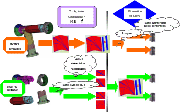
Figure 3.2-1._ MUMPS centralized/distributed data flows/parallel processing.

3.2.2. Different distribution methods

This paragraph describes the various choices for distributing elementary calculations to the processors participating in the calculation. This distribution is adjusted during the construction of the finite element model.

A first choice is not to distribute elementary calculations between processors. If you want to distribute the elementary calculations, you can rely on a distribution of finite elements or a distribution of cells (regardless of the finite elements carried by these cells). Finally, it is possible to combine distribution by finite element and by mesh. Let’s detail each mode:

• CENTRALISE: The stitches are not distributed (as in sequential). Elementary calculations are not parallelized. Parallelism only starts at the MUMPS level. Each processor builds and provides the linear solver with the entire system to be solved. This mode of use is useful for non-regression testing. In all cases where elementary calculations represent a small part of the total time (e.g. in linear elasticity), this option may be sufficient.

“ GROUP_ELEM”: * A second type of distribution consists in forming homogeneous groups of finite elements (by type of finite element) and then in distributing the elementary calculations between the processors to best balance the load (in terms of the number of elementary calculations of each type). Each processor allocates the entire matrix but only performs and assembles the elementary calculations that have been assigned to it.

• “ MAIL_DISPERSE/MAIL_CONTIGU “ :

The cells of the model are distributed either by contiguous cell packs (“MAIL_CONTIGU”), or by cyclic distribution (“MAIL_DISPERSE”). This distribution is independent of the type of finite element carried by the meshes. For example, with a model comprising 8 cells and for a calculation on 4 processors, we have the following load distributions:

Distribution method	Mesh 1	Mesh 1	Mesh 2	Mesh 3	Mesh 5	Mesh 6	Mesh 6	Mesh 7	Mesh 7	Mesh 7	Mesh 8
MAIL_CONTIGU	Proc. 0	Proc. 0	Proc. 0	Proc. 0	Proc. 0	Proc. 0	Proc. 0	Proc. 3	Proc. 3	Proc. 3
MAIL_DISPERSE	Proc. 0	Proc. 1	Proc. 1	Proc. 2	Proc. 3	Proc. 0	Proc. 1	Proc. 2	Proc. 2	Proc. 3

Each processor allocates the entire matrix but only performs and assembles the elementary calculations that have been assigned to it.

• “ SOUS_DOMAINE “(default): This type of distribution is a hybrid distribution of elementary calculations based on a distribution of cells (based on a partitioning of the global mesh into sub-domains) then on a distribution of finite elements by type within each sub-domain. Each processor allocates the entire matrix but only performs and assembles the elementary calculations that have been assigned to it.

3.2.3. Load balancing

The distribution by cells is very simple but can lead to load imbalances because it does not explicitly take into account spectator cells, skin elements (cf. figure 3.2-2 on an example comprising 8 volume cells and 4 skin elements), particular areas (non-linearities…). Distribution by sub-domains is more flexible and can be more effective by allowing you to adapt your data flow to your simulation.

Another cause of imbalance may come from Dirichlet conditions by dualization (DDL_IMPO, LIAISON_ **…). For reasons of robustness, their processing is assigned only to the master processor. This workload, which is often negligible, introduces, however, in some cases, a more pronounced imbalance. The user can compensate for it by entering one of the CHARGE_PROC0_MA /SD keywords. This differentiated treatment in fact concerns all cases involving so-called « late » meshes (Dirichlet*via Lagrange multipliers but also nodal force, contact continuous method…).

For more details on the computer specifications and the functional implications of this mode of parallelism, you can consult the documentation [U2.08.03] and [U4.50.01].

Notes:

• Without the option MATR_DISTRIBUEE (see next paragraph), the different strategies are equivalent in terms of memory occupancy. The flow of data and instructions is being dried up as soon as possible. It is a question of selectively dealing with the matrix/vector blocks of the global problem, which MUMPS will bring together.

• In distributed mode, each processor only manipulates partially filled matrices. On the other hand, in order to avoid introducing too many MPI communications into the code (stopping criteria, residue…), this scenario was not retained for the second members. Their construction is well parallelized, but at the end of assembly, the contributions of all the processors are summed up and sent to everyone. So all processors fully know the vectors involved in the calculation.

• Likewise, the matrix is currently duplicated: in space JEVEUX (RAM or disk) and in space F90 of MUMPS (RAM). In the long run, due to the unloading of the factorized one onto disk, it will become a dimensioning object of the RAM. It will therefore have to be built directly via MUMPS.

3.2.4. Resize Code_Aster objects

In parallel mode, when distributing data JEVEUX upstream of MUMPS, you do not necessarily recut the data structures concerned. With the option MATR_DISTRIBUEE =” NON “, all distributed objects are allocated and initialized at the same size (the same value as sequentially). On the other hand, each processor will only modify the parts of objects JEVEUX for which it is responsible. This scenario is particularly suited to the distributed parallel mode of MUMPS (mode by default) because this product groups these incomplete data streams internally. Parallelism then makes it possible, in addition to saving in calculation time, to reduce the memory space required by resolution MUMPS but not that required to build the problem in JEVEUX.

This is not a problem as long as RAM space for JEVEUX is much less than that required by MUMPS. Since JEVEUX mainly stores the matrix and MUMPS stores its factored (usually dozens of times bigger), the calculation bottleneck RAM is theoretically on MUMPS. But as soon as you use a few dozen processors in MPI and/or activate OOC, as MUMPS distributes this factorized by processor and unloads these pieces onto disk, the « ball comes back into the court of JEVEUX ».

Hence option MATR_DISTRIBUEE, which resizes the matrix, more precisely non-zero terms for which the processor is responsible. The JEVEUX space required then decreases with the number of processors and falls below the RAM required at MUMPS. The results in Figure 3.2-2 illustrate this gain in parallel on two studies: a Pump RIS and a tank model from the « Epicure » study.

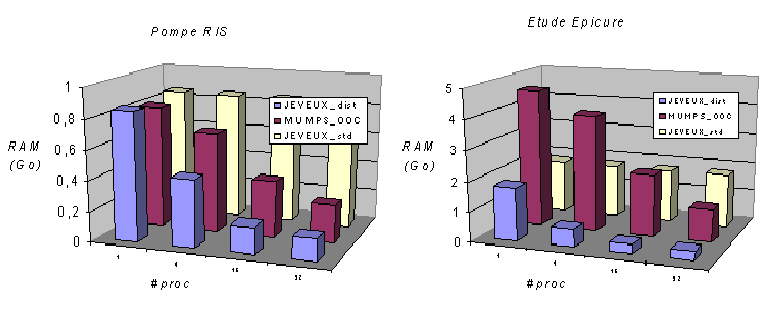
Figure 3.2-2._Evolution of consumption RAM (in GB) according to the number of processors, Code_Aster v11.0 ( JEVEUX standard MATR_DISTRIBUE =” NON “and distributed, resp.” OUI “) and MUMPS OOC. Results carried out on a RIS Pump and on the Epicure study tank.

Notes:

• Here we treat data resulting from an elementary calculation (RESU_ELEM and CHAM_ELEM) or from a matrix assembly (MATR_ASSE). The assembled vectors (CHAM_NO) are not distributed because the memory gains induced would be low and, on the other hand, as they are involved in the evaluation of numerous algorithmic criteria, this would involve too many additional communications.

• In mode MATR_DISTRIBUE, to make the join between the end of MATR_ASSE * local to the processor and the global MATR_ASSE (which we do not build), we add an indirection vector in the form of a NUME_DDLlocal.

3.3. Memory Management MUMPS and Code_Aster

To activate or deactivate the OOC abilities of MUMPS (cf. figure 3.3-1), ** the user enters the keyword SOLVEUR/GESTION_MEMOIRE =” IN_CORE “/” OUT_OF_CORE “/” AUTO “(default). This functionality can of course be combined with parallelism, resulting in a greater variety of operations to possibly adapt to execution contingencies: « sequential IC or OOC », « centralized parallelism IC or OCC », « parallelism distributed by sub-domains IC or », « parallelism distributed by sub-domains IC or OOC »…

For a small linear case, the « sequential IC » mode is sufficient; for a larger case always in linear mode, the « centralized parallel IC » mode (or better OOC) really brings a gain in CPU and RAM; in non-linear, with frequent updating of the tangent matrix, the « distributed parallel OOC » mode is recommended.

For more details on the computer specifications and the functional implications of this mode of memory management MUMPS we can consult the documentation [BD08] and [U2.08.03/U4.50.01].

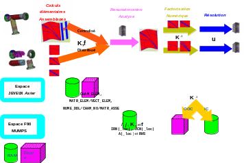
Figure 3.3-1._ Functional diagram of the Code_Aster/ MUMPS coupling (with a sequential renumber)

with respect to the main data structures and memory occupancy (RAM and disk) .

3.4. Special management of double Lagrange multipliers

Historically, Code_Aster’s direct linear solvers (“MULT_FRONT” and “LDLT”) did not have a pivoting algorithm (which seeks to avoid the accumulation of rounding errors by division by very small terms). To get around this problem, the consideration of limit conditions by Lagrange multipliers (AFFE_CHAR_MECA/THER…) has been modified by introducing Lagrange double multipliers. Formally, we do not work with the initial matrix K 0

\({\mathrm{K}}_{0}\mathrm{=}\left[\begin{array}{cc}\mathrm{K}& \mathrm{blocage}\\ \mathrm{blocage}& 0\end{array}\right]\begin{array}{c}\mathrm{u}\\ \mathrm{lagr}\end{array}\)

but with its doubly dualized form K 2

\({\mathrm{K}}_{2}\mathrm{=}\left[\begin{array}{ccc}\mathrm{K}& \mathrm{blocage}& \mathrm{blocage}\\ \mathrm{blocage}& \mathrm{-}1& 1\\ \mathrm{blocage}& 1& \mathrm{-}1\end{array}\right]\begin{array}{c}\mathrm{u}\\ {\mathrm{lagr}}_{1}\\ {\mathrm{lagr}}_{2}\end{array}\)

Hence an additional memory and calculation cost.

As MUMPS has pivoting capabilities, this choice to dualize boundary conditions can be called into question. By initializing the keyword ELIM_LAGR to “LAGR2”, we only take into account one Lagrange, the other being a spectator [34] _ . Hence a \({K}_{1}\) work matrix that is simply dualized.

\({\mathrm{K}}_{1}\mathrm{=}\left[\begin{array}{ccc}\mathrm{K}& \mathrm{blocage}& 0\\ \mathrm{blocage}& 0& 0\\ 0& 0& \mathrm{-}1\end{array}\right]\begin{array}{c}\mathrm{u}\\ {\mathrm{lagr}}_{1}\\ {\mathrm{lagr}}_{2}\end{array}\)

smaller because the extra-diagonal terms of the rows and columns associated with these spectator Lagrange multipliers are then initialized to zero. *Conversely, with the value “NON”, MUMPS receives the usual dualized matrices.

For problems with numerous Lagrange multipliers (up to 20% of the total number of unknowns), activating this parameter is often expensive (smaller matrix). But when this number explodes (> 20%), this process can be counterproductive. The gains made on the matrix are cancelled out by the size of the factorized one and especially the number of late pivots that MUMPS must perform. Imposing ELIM_LAGR =” NON “can then be very interesting (gain of 40% in CPU on the mac3c01 test case).

3.5. Scope of use

Priori, all operators/functionalities using the resolution of a linear system except a modal calculation configuration [35] _ . For more details you can consult the User documentation [U4.50.01].

3.6. Parameterization and examples of use

Let’s summarize the main configuration for controlling MUMPS in Code_Aster and illustrate its use via an official test case (mumps05b) and a study geometry (pump RIS). For more information you can consult the associated user documentation [U2.08.03/U4.50.01], the notes EDF [BD08] [] [Boi07] [Des07] or the test cases using MUMPS.

3.6.1. Parameters for using MUMPS ViaCode_aster

Table 3.6-1._ Summary of the specific setting of MUMPS in Code_Aster.

3.6.2. Monitoring

By positioning the keyword INFOà 2 and using the MUMPS solver, the user can have a summary monitoring of the various phases of the construction and resolution of the linear system displayed in the message file: distribution by processor of the number of cells, terms of the matrix and its factorized form, error analysis (if requested) and an assessment of their possible imbalance. To this CPU oriented monitoring, we add some information on the RAM consumption of MUMPS: by processor, estimate (according to the analysis phase) of the needs in RAM in IC, in OOC and the value actually used with a reminder of the strategy chosen by the user. The times consumed for each of the steps of the calculation according to the processors may also appear. They are managed by a more global mechanism that is not specific to MUMPS (see §4.1.2 [U1.03.03] or the User documentation for the DEBUT/POURSUITE operator).

---

<DNT_dlijmjenlhenkknhafchjikfnfagbcam MUMPS >

TAILLE FROM SYSTEME 803352

CONDITIONNEMENT/ERREUR ALGO 2.2331D+07 3.3642D-15

ERREUR SUR THE SOLUTION 7.5127D-08

RANG **** NBRE MAILLES **** NBRE TERMES K LU FACTEURS

N 0:54684 7117247 117247 117787366

N 1:55483 7152211 90855351

…

IN%: VALEUR RELATIVE AND DESEQUILIBRAGE MAX

: 1.45D+01 2.47D+00 2.38D+00 1.50D+01 4.00D+01 2.57D+01

: 1.40D-01 -1.09D+00 -5.11D+00 -5.11D+00 -9.00D-02 1.56D+00 -4.16D-01

MEMOIRE RAM ESTIMEE AND REQUISE **** PAR MUMPS EN MB (FAC_NUM + RESOL)

MASTER RANK: ESTIM IN-CORE | ESTIM OUT-OF-CORE | RESOLVED. OUT-OF-CORE

NO. 0:1854 512 512

N 1:1493 482 482

…

#1 Resolution of linear systems CPU (USER + SYST//SYST/ELAPS): 105.68 3.67 59.31

#1 .1 Numbering, matrix connectivity CPU (USER + SYST/SYST/ELAPS): 3.26 0.04 3.26

#1 .2 Symbolic factorization CPU (USER + SYST//SYST/ELAPS): 3.13 1.20 4.11

#1 .3 Numerical factorization (or precond.) CPU (USER + SYST/SYST/ELAPS): 45.22 0.83 23.48

#1 .4 Resolution CPU (USER + SYST/SYST/ELAPS): 54.07 1.60 28.46

#2 Elementary calculations and assemblies CPU (USER + SYST/SYST/ELAPS): 3.44 0.03 3.42

#2 .1 Routine calculation CPU (USER + SYST//SYST/ELAPS): 2.20 0.01 2.20

#2 .1.1 Routines te00ij CPU (USER + SYST//SYST/ELAPS): 2.07 0.00 2.06

#2 .2 Assemblies CPU (USER + SYST//SYST/ELAPS): 1.24 0.02 1.22

#2 .2.1 Assembling matrices CPU (USER + SYST//SYST/ELAPS): 1.22 0.02 1.21

#2 .2.2 Assembling second members CPU (USER + SYST//SYST/ELAPS): 0.02 0.00 0.01

Figure 3.5-1. _Excerpt from message file in INFO =2.

3.6.3. Examples of use

Let’s conclude this chapter with two series of tests illustrating the performance differences depending on the case and the observed criterion (cf. figures 3.5-2/3). The canonical linear cube test case parallelizes very well. In centralized (or distributed), more than 96% (resp. 98%) of the construction and inversion phases of the linear system are parallelized. That is to say a theoretical speed-up close to 25 (resp. 50). In practice, on the parallel nodes of the centralized Aster machine, we obtain fairly good accelerations: effective speed-up of 14 out of 32 processors instead of the theoretical 17.

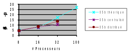
\(N\mathrm{=}0.7M\mathrm{/}\mathit{nnz}\mathrm{=}27M\)

%parallel centralized/distributed: 96/98

Theoretical speed-ups hundred. /dist. <25/50

32 proc (x1): ~3min

Conso. RAM IC: 4GB (1 proc) /1.3GB (16)

Conso. RAM OOC: 2GB (1 proc) /1.2GB (16)

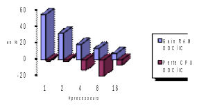
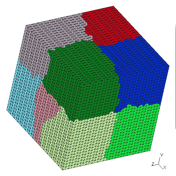
Figure 3.5-2._ Linear mechanical calculation (op. MECA_STATIQUE) on the official cube test case (mumps05b). We build and solve a single linear system. Simulation performed on the centralized Aster machine with Code_Aster v11.0. Consumption RAM Aster+ MUMPS measured.

On the non-linear study of the pump, the gains that can be expected are lower. Given the sequential analysis phase of MUMPS, only 82% of the calculations are parallel. Hence, significant but more modest theoretical and effective speed-ups. From a memory point of view RAM, the OOC management of MUMPS provides interesting gains in both cases, but more pronounced for the pump: sequentially, gain IC vs OOC of the order of 85%, against 50% for the cube. By increasing the number of processors, the data distribution that parallelism induces progressively reduces this gain. But it remains prominent on the pump up to 16 processors and almost disappears with the cube.

\(N\mathrm{=}0.8M\mathrm{/}\mathit{nnz}\mathrm{=}28.2M\)

%parallel centralized/distributed: 55/82

Theoretical speed-ups hundred. /dist. <3/6

16 times ~15 min

Conso. RAM IC: 5.6GB (1 proc) /0.6GB (16)

Conso. RAM OOC: 0.9 GB (1 proc) /0.3 GB (16)

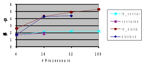
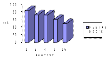
Figure 3.5-3._ Nonlinear mechanical calculation (op. STAT_NON_LINE) on a more industrial geometry (RIS pump). We build and solve 12 linear systems (3 time steps x 4 Newton steps). Simulation performed on the centralized Aster machine with Code_Aster v11.0. Estimated RAM MUMPS consumptions.

[1]

This continuous search for improved performance is obviously not limited to linear solvers alone. The code offers a number of tools to meet the same objectives: distribution of independent calculations, X- FEM, improvement of touch-friction, EDO /modal/non-linear solvers, adaptive meshing, finite structural elements…

[2]

Cf. [R6.01.03] for a detailed view of potential parallelism strategies and those actually implemented in the code.

[3]

To maintain the consistency of data structures and maintain a certain computer readability/maintainability, it is better to « bluff » the usual process by moving from \({K}_{2}\) to \({K}_{1}\), rather than to the optimal scenario \({K}_{0}\).

[4]

Solving a quadratic problem with CALC_MODES + OPTION =” SEPARE “/” AJUSTE “. Because this option requires direct access to the diagonal of the factored matrix. However, MUMPS does not allow, for the moment, to know the precise terms of the factored value actually obtained. On the other hand, and this is his preferred framework of use, he uses them effectively and with robustness to solve a linear system and/or to calculate a post-treatment (Sturm criterion, determinant calculation, etc.).