7. Appendix 1: Principle of compressions BLR in MUMPS#

This paragraph summarizes the various technical aspects of thesis work by Clément Weisbecker on low-rank compressions [CW15] [Boi13]. This work has been continued and improved by the MUMPS team and is partly available in the consortium version [MUC] of the product.

For more details you can consult the thesis document itself [CW13]. The figures reused here come from elsewhere, either from this document or from the slide deck from his defense.

Principle of the multifrontal method

The multifrontal method is a direct method class used to solve linear systems. It is this method that is implemented in product MUMPS and it is it that is generally used in major commercial codes in structural mechanics (ANSYS, NASTRAN…). Even if there are other strategies (supernodal…) and they are beginning to be implemented in public packages (SuperLU, PastiX…), this thesis work focused exclusively on this standard strategy that is multifrontend. Nevertheless, many of its results can undoubtedly be extended or adapted to these other resolution methods.

The multifrontal method, developed by I.S.Duff and J.K.Reid (1983), consists in particular in using graph theory [38] _ to build, from a sparse matrix, a elimination tree that efficiently organizes the calculations (cf. figures 7.1.1). Black squares represent non-zero matrix terms. To manipulate, « by interposed graphs », this type of data, the following rule is usually imposed: a point on the graph represents an unknown and, an edge between two points, a non-zero matrix term.

So in the example below, variables 1 and 2 must be connected by an edge (in the initial numbering). Generally, the initial matrix numbering is not optimal. In order to reduce the memory footprint of the factorized [39] _ , the number of flops of subsequent manipulations and in order to try to guarantee a good level of precision of the result, we renumber this initial matrix. We can thus see that the number of additional terms (“fill-in”) created by factorization increases from 16 to 10.

It is from this renumbered matrix that the elimination tree specific to the multifrontal is constructed. This tree-like vision has the great merit of organizing the tasks concretely: we precisely determine their dependency or not (to maintain parallelism), their precedence e (to make groupings in order to optimize performance BLAS); we can predict certain consumption (in time and memory) or even try to limit numerical problems.

Thus, in the example below, the treatment of variable 1 has no impact on variables 2, 4, and 5. On the other hand, it will impact variables 3 and 7 that occupy the upper levels of the tree (they are its ascendants).

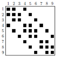
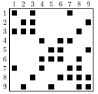
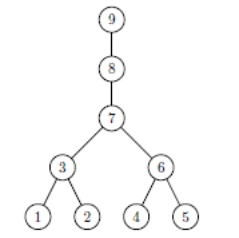
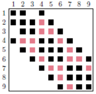
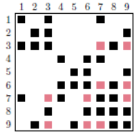
Figure 7.1.1_ First line, from left to right: an initial sparse matrix, the same reordered matrix, and the elimination tree associated with it. Second line, from left to right: the factored ones corresponding to the initial and renumbered matrices.

The second strong idea of the multidisciplinary method is to bring together a maximum of variables (we speak of amalgamation) in order to constitute « fronts » (dense) whose numerical processing will be much more efficient (via via BLAS routines).

Even if it means filling the corresponding matrix sub-block with real zeros and manipulating them as is [40] _ . For example, this is what is done in the tree in Figure 7.1.2 between the amalgamated variables 7, 8 and 9. There are numerous amalgamation techniques based on graph criteria, numerical aspects, or computer considerations (e.g. distributed parallelism).

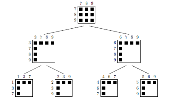
Figure 7.1.2_ Elimination tree with matrix blocks and a choice of « fronts » .

Note:

For the sake of simplification, we will not discuss in this summary the other numerical treatments that are often involved in the process: scaling terms (“scaling”), permutation of columns and static/dynamic pivoting. As the « devil is often in the details », it is however these related treatments that have complicated Clément’s numerical work and computer developments. They are essential to the smooth running of many of our industrial simulations with Code_Aster.

7.1. Elimination tree#

Algorithmic processing of the tree starts from the bottom (at the level of the « leaves ») to the top (towards « the root »). Within each leaf or each branch « node » we associate a dense front. In a front, two types of variables are distinguished:

“Fully Summed” (FS) which, as their name suggests, are completely processed and will no longer be updated;
the “Non Fully Summed” (NFS) who they are always waiting for contributions from other branches of the tree.

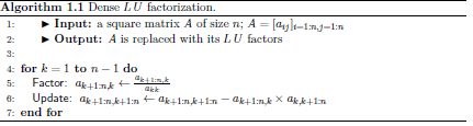
The first type of variables can be completely « eliminated »: the terms of the factored matrix concerning them (rows of**U**and columns of**L) are calculated and stored [41] _ once and for all. The second type produces a block of contributions [42] _ (noted CB for “Contribution Blocks”) which will be added at the top level of the tree with other CBs associated with the same variables (cf. figure 7.2.1).

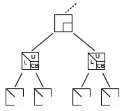
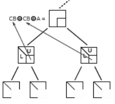
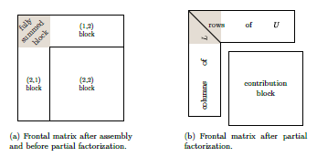
Figure 7.2.1_ General structure of a « front » before and after treatment.

In turn, some variables associated with these blocks will be eliminated and others, on the contrary, will continue to participate actively in the process by providing CBs again. And so on… all the way to the root of the tree. At this last stage, there are only variables eliminated and no more CB!

Thus, in the fronts associated with the leaves on the left in Figure 7.2.1, the variables 1 and 2 are FS, while the variables 3, 7 and 9 are NFS. The latter provide CBs that will be accumulated in the upper level front combining the variables 3, 7, 8 and 9. The latter will « relieve » the algorithmic process of the FS 3 variable (it will be eliminated), while NFS 7, 8 and 9 will continue their journey through the tree.

7.2. Algorithmic treatments#

In the case of a general dense matrix A, Gauss factorization leads to iteratively constructing the terms of L and those of U according to an algorithm of type 1.1 (cf. figure 7.3.1). Here, to simplify, we do not take into account terms that are null (or too small), nor numerical aspects such as pivoting, permutation or scaling.

Each step k corresponds to a pivot (assumed to be non-zero) which will lead to the updating of the block

underlying, as well as the construction of the column and the corresponding row of L and U.

This algorithm therefore requires two types of operations:

A factorization step (noted as” Factor “) that uses the diagonal pivot

to build the k -th part of the factored one and thus eliminate the k -th variable (it will be called FS).

A update step (noted “Update”) that builds the contribution block (CB).

The algorithmic complexity of the set and its memory cost are respectively in

And in

. These figures alone illustrate the impact of this stage on the performance of our simulations (even if they are carried out in “sparse”).

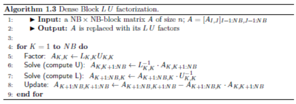
Algorithms 7.3.1_ Examples of dense, scalar and block factorization algorithms.

In order to optimize costs we generally work on blocks and not on scalars (cf. algorithm 1.3). The data to be collected in memory RAM, at the same time, is smaller in size and vector and matrix algebraic operations are much more efficient (via optimized BLAS routines).

The types of operations to be performed remain the same:

Local factorizations of diagonal blocks (”Factor”),
Descent-lifts (noted “Solve”) to effectively build the column/line blocks of the factorized one,
Update (”Updat e”) by blocks of the sub-matrix.

In the elimination trees presented above, this type of operation is carried out within each front, then between each front and its « father ». The objective of low-rank compression will be to reduce their algorithmic complexity as well as their memory footprint (peak RAM and disk consumption).

7.3. Memory Management#

On this last point, often the most crucial for our studies, t**the whole problem lies in the « delayed management of CBs »**. During the k step of algorithm 1.3, you must keep in RAM not only the « active » front, but also the CBs waiting to be processed and the (possible) factors not unloaded on disk (if the OOC is activated). They constitute the active memory of the process (blue and green area in Figure 7.4.1).

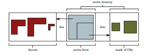
Figure 7.4.1_ Memory management of the various elements handled by the multifront end.

This active memory is managed like a stack. It fluctuates constantly. It believes when a front is loaded. Then it decreases as CBs associated with this front are consumed. Finally, it recovers with the new factors and the new CB resulting from this front.

The new factors are then possibly copied onto disk. The memory footprint of these factors (red zone on the left of the graph) is easier to analyze: it only swells as the tree goes up!

In any case, these two memory areas are not easy to predict a priori. They depend in particular on renumbering, on the construction of the elimination tree but also on numerical pretreatments. This is one of the tasks performed by the analysis stage in MUMPS. It is useful both for the multifront end to allocate its memory areas efficiently, but also for the calling code in order to better manage its own internal objects [43] _ . The optimized management of these elements is further complicated due to numerical treatments that are carried out dynamically during factorization: for example, the organization of pivoting and the distribution of data in parallel.

It is the peak of this active memory that constitutes the essential challenge of this thesis. It is often much greater than the size of the factored one. However, it is already often in 500N in our current studies (with N the size of the problem). Thus, the processing of a matrix comprising 1 million unknowns requires at least 500*1*12 [44] _ =6GB of RAM (in real double precision). And this figure tends to increase with the size of the problem (we go from 500N to 1000N or even more).

We can therefore reach peaks RAM that even parallel data distribution combined with OOC will not be able to manage effectively [45] _ . So any significant reduction in this peak would be a very significant gain for our current and future major studies.

7.4. Low-rank approximation#

A dense matrix A, of size m x n, is said to be « low-rank » (“low-rank”) of order k (< min (m, n)) *) when it can be decomposed as

(7.5-1)

with U and V much smaller matrices (respectively m x k and k x*n*) and E a « negligible » m x*n* matrix (

). This notion of « numerical rank » should not be confused with the concept of algebraic rank.

During subsequent manipulations, the approximation is then made

(7.5-2)

by betting (often under control), that it will have little impact on the overall process. This approximation is therefore dependent on the compression parameter*e*.

It is this parameter that we will vary, in practice, to adapt the low-rank gains to the situation. For example:

with e<10-9 we have compression with a slight and controllable loss of precision. We can of course continue to use the multifrontend as a direct solver. To regain precision identical to the full-rank case, one or two iterations of iterative refinement are sufficient [46] _

with e>10-9 compression is better but the loss of precision can be significant [47] _

. We can then use the factored one to build a preconditioner, more or less « frustrating », speeding up an iterative Krylov solver.

On the other hand, apart from obvious gains in terms of storage, the manipulation of such matrices can prove to be very advantageous: the rank of the sum is less (at worst) than the sum of the ranks and the rank of the product is lower than the minimum of the ranks. Once decomposed, the manipulation of low-rank matrices can therefore be (relatively) controlled in order to optimize the compression of the result.

So the product of two dense matrices of size n x n and of rank k, with

, reduces the an algorithmic complexity of the operation of

unto

; her memory imprint passing from

unto

A matrix transformed into low-rank form is called « downgraded » (”demoted”) or compressed. The inverse transformation, except for approximations, « promotes » the matrix (”promoted”) or the decompress.

To keep the same terminology when handling a matrix in a standard way (without exhibiting a decomposition of the type (7.5-1)), we say that it is of full rank (“full-rank”).

The « low-rank decomposition » of a matrix can be done in various ways:

SVD,
Rank-Revealing QR (RRQR),
Adaptive Cross Approximation (ACA),
Random sampling.

In this thesis Clément mainly uses the second solution, which is less accurate than a classic SVD but much less expensive. The main thing is that this compression is shared between different treatments and that it allows maximum compression. Ideally, the rank obtained should therefore satisfy a condition of the type:

(7.5-3)

Part of Clément’s work consisted in developing heuristics adapted to multifrontend in order to try to respect this criterion as often as possible.

7.5. “Block Low-Rank” Multifrontal (BLR)#

The objective of this thesis is to exploit this type of compression by decomposing the largest fronts of the elimination tree of a multifrontal in low-rank form. Because it is these dense matrix sub-blocks that generate the most flops and that hinder peak RAM (because of all the CBs that they will agglomerate). In general, these large fronts are located in the last levels of the elimination tree.

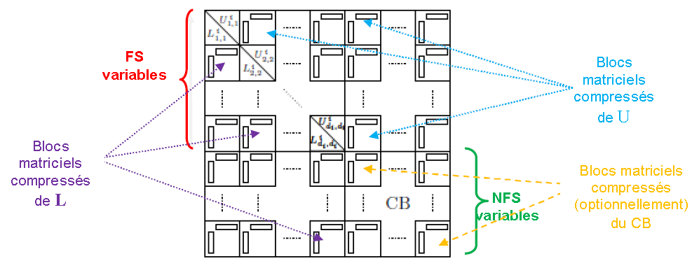
Figure 7.6.1_ Structure of a compressed edge after factorization.

As illustrated below (cf. figure 7.6.1) we will therefore, firstly, break down into columns and rows of sub-blocks (decomposition by “panels”), the matrix blocks corresponding to the four types of front terms (according to the terminology in Figure 7.2.1):

FSxFS (“block (1,1) “),
FSxNFS (“block (1.2) “),
NFSxFS (“block (2,1) “),
NFSxNFS (“block (2,2) “).

Then each of these sub-blocks will be compressed in low-rank according to the formula (7.5-1). At least when this compression is legal [48] _ . Except for the diagonal sub-blocks in sub-part FSxFS which remain in full-rank (to optimize their subsequent manipulations).

We adapt the size of the panels so that it is:

Large enough to take advantage of the performance of BLAS kernels (loop invariant, minimization of cache faults and optimized management of the memory hierarchy);
Not too large to provide flexibility in subsequent numerical (pivoting, scaling) and computer (distributed parallelism) manipulations;
Medium-size in order to optimize MPI communication costs (latency*verse* bandwidth).
Medium-size in order to provide flexibility in the grouping of variables that will follow (the “clustering”). This reorganization should generate maximum compression.
Not too big to not cost too much in SVD or RRQR.

But the whole problem lies in the fact that these matrix sub-blocks have no reason to be low-rank! Even if they are large in size, the parts of “demoted” fronts can be full in rank. The costs of SVDs or RRQRs will then not be compensated and the compression objective will be compromised!

Inspired by the work already done by other compression techniques (hierarchical matrices of type H, H2, HSS/SSS…), criteria have been developed to decompose the variables composing a front and renumber them so that they generate low-rank matrix sub-blocks. This criterion is based on the following empirical finding:

The more distant two variable blocks are, the lower the numerical rank of the matrix block it involves becomes.

This condition called « eligibility » was tested on some model problems resulting from the discretization of elliptical EDP and is illustrated in Figure 7.6.2. With the terminology of graph theory it can be reformulated in the following form:

(7.6-1)

with*diam* and dist, the usual notions of diameter and distance in the graph associated with the treated edge.

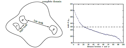
Figure 7.6.2_ Evolution of the « numerical » rank of two groups of variables of homogeneous size as a function of the distance (in the sense of the graphs) that separates them.

Thus, in the example in the figure below (cf. figure 7.6.3), by dividing the front variables into slices, an increase in the number of terms of 17% is obtained. That is to say that, on average, each sub-block admits a numerical rank k such that

Whereas with checkerboard cutting, the gain reaches 47%:

. This difference is due to the greater regularity of the second over the first. Homogeneous square-shaped sub-blocks have diameters that are rapidly smaller than the distance between sub-blocks. With their elongated shape, this is obviously not the case with sub-blocks resulting from slicing!

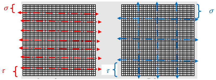
Figure 7.6.3_ Example of two types of clustering on a dense front: slice and checkerboard.

7.6. A few additional elements#

It is therefore on an eligibility criterion of this type that MUMPSt will base its clustering of the variables composing a front. He worked hard to make this « key operation » of the method compatible with the digital-computer constraints of the multifrontend and the MUMPS tool; while ensuring maximum compression and limiting its additional cost (in time).

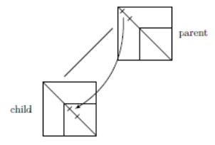
Figure 7.7.1_ « Inherited » clustering between variables NFS from a front

and those FS from an anterior front.

Example of sophistication: this clustering is operated separately on the two types of variables, FS and NFS. As when going through the elimination tree, the variables NFS of a front become the FS of the fronts of the higher levels, we break down this task. On the other hand, these cuts are not completely repeated at each front. Some information is shared in order to limit additional costs (in time). This particular clustering algorithm is called « inherited » (“inherit”) **as opposed to the**standard algorithm called « explicit » ** for which the two clusterings are repeated at each manipulation again.

The additional cost of the « explicit » clustering variant can be prohibitive for very big problems (several times the cost of the entire analysis phase!) while the cost of optimized clustering remains reasonable: only a few percent of this analysis phase. The low-rank gains of the two variants are very similar, but the implementation of the optimized version is more complex.

Finally, these clusterings are performed by standard tools, METIS or SCOTCH. But they are not applied directly to the variables of the fronts but to halos encompassing them. This trick makes it possible to properly orient these divisions so that they produce groups of contiguous homogeneous nodes.

On the other hand, to be more precise, the treatment of an forehead comprises five steps (already mentioned in the algorithms in FIG. 7.3.1). We start by dividing the variables into two levels interlocked with panels:

the first level, the largest, the one that is outside (called “outer panel” or “BLR panel”), results from low-rank clustering;
while the second, the one inside the previous one (”inner panel” or “BLAS panel”) groups the variables into sub-packages of 32, 64 or 96 contiguous variables in order to feed the computing cores more efficiently (and reduce the cost of MPI communications and I/Os).

Then, we have two interlocked loops: the first on panels BLR and the second on panels BLAS. For a given panel BLAS, we perform:

the factorization step (F),
the Solve stage (S),
the Internal Upgrade (UI) between all the following sub-panels of panel BLR,
the External Upgrade (UE) between all the following BLR panels.

The standard order of operations can therefore be roughly noted FSUU . Depending on the level at which low-rank compression (**C) is used, we then distinguish 4 variants:

FSUUC,
FSUCU,
FSCUU,
FCSUU.

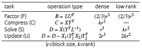
Table 7.7.2_ Comparison of the costs of the various stages

in dense (full-rank) and in low-rank.

It is variant No. 3, FSCUU, that industrialized the consortium versions of MUMPS.

Given the relative costs of each of the operations (cf. table 7.7.2) and the tool robustness constraints, it is this variant that was favored. It makes it possible to significantly reduce overall costs while maintaining maximum precision in the first two steps (F and S). Because these are crucial in the management of several sophisticated digital ingredients (scaling, pivoting, singularity detection, determinant calculation, Sturm test…). Initially, it was therefore preferred to impact them as little as possible by this compression. So this is done just after. And its gains (and any approximations) will only impact internal and external updates (UI and EU).