1. Overview of direct solvers#
1.1. Linear system and associated resolution methods#
In numerical simulation of physical phenomena, a significant computational cost often comes from the construction and resolution of linear systems. Structural mechanics is no exception to the rule! The cost of building the system depends on the number of integration points and on the complexity of the laws of behavior, while that of solving is linked to the number of unknowns, to the models used and to the topology (width of the band, conditioning). When the number of unknowns explodes, the second step becomes preponderant [1] _ and it is therefore the latter that will mainly interest us here. Moreover, when it is possible to be more efficient in this resolution phase, thanks to access to a parallel machine, we will see that this advantage can be propagated to the phase of constitution of the system itself (elementary calculations and assemblies).
These inversions of linear systems are in fact omnipresent in codes and often buried in the depths of other numerical algorithms: non-linear schema, time integration, modal analysis… For example, we are looking for the vector of nodal displacements (or displacement increments) \(u\) verifying a linear system of the type
\(\mathrm{Ku}\mathrm{=}\mathrm{f}\) (1.1-1)
with \(K\) a stiffness matrix and \(\mathrm{f}\) a vector representing the application of generalized forces to the mechanical system.
In general, the resolution of this type of problem requires a (more) broad question than it seems:
Do we have access to the matrix or do we simply know its action on a vector?
Is this matrix hollow or dense?
What are its numerical properties (symmetry, positive definition…) and structural properties (real/complex, by bands, by blocks…)?
Do we want to solve a single system (1.1-1), several simultaneously [2] _
or consecutively [3] _ ? Even several different and successive systems whose matrices are very similar [4] _ ?
In the case of successive resolutions, can we reuse previous results in order to facilitate future resolutions (cf. restart technique, partial factorization)?
What is the order of magnitude of the size of the problem, of the matrix and of its factorized in relation to the processing capacities of CPU and associated memories (RAM, disk)?
Do we want a very precise solution or simply an estimate (cf. nested solvers)?
Do we have access to linear algebra libraries (and their prerequisites MPI, BLAS, LAPACK…) or should we use « homemade » products?
In Code_Aster, we explicitly build the matrix and store it in the format MORSE [5] _ . With most models, the matrix is sparse (due to discretization by finite elements), potentially poorly conditioned [6] _
and often real, symmetric, and indefinite [7] _ . In non-linear, modal or thermo-mechanical combinations, problems such as « multiple second members » are often treated. Discrete contact and friction methods take advantage of partial factorization capabilities and the domain decomposition method. On the other hand, Code_Aster also uses simultaneous resolution scenarios (Schur complements of contact and substructuring…).
As for the sizes of the problems, even if they increase from year to year, they remain modest compared to CFD: in the order of a million unknowns but for hundreds of steps of time or Newton iterations.
Moreover, from a « middleware and hardware » point of view, the code is now based on numerous optimized and sustainable libraries (MPI, BLAS, LAPACK, (PAR) METIS, (PT) SCOTCH, PETSc, MUMPS…) and is mainly used on clusters of SMP (fast networks) , large storage capacity RAM and disk). The main aim is therefore to optimize the use of linear solvers in this perspective.
For 60 years, two types of techniques have been competing for supremacy in the field, direct solvers and iterative solvers (cf. [Che05] [Dav03] [Duf06] [Gol96] [Las98] [Las98] [Las98] [Las98] [Liu89] [Liu89] [Meu99] [Saa03]).
The first ones are robust and result in a finite number of operations (theoretically) known in advance. Their theory is relatively well completed and their variation according to many types of matrices and software architectures is very complete. In particular, their multi-level algorithms are well adapted to the memory hierarchies of current machines. However, they require storage capacities that grow rapidly with the size of the problem, which limits the scalability of their parallelism. [8] _ . Even if this parallelism can be broken down into several independent layers, thus increasing performance.
On the other hand, iterative methods are more « scalable » when the number of processors is increased. Their theory is full of numerous « open problems », especially in finite arithmetic. In practice, their convergence into a « reasonable » number of iterations is not always acquired, it depends on the structure of the matrix, the starting point, the stopping criterion… This type of solvers has more difficulty in breaking through industrial structures in mechanics where we often combine heterogeneities, non-linearities and model junctions that complicate the conditioning of the work operator. On the other hand, they are not adapted to effectively solve « multiple second member » problems. Except these are very common in the algorithmic of mechanical simulations.
Figure 1.1-1._ Two classes of methods for solving a linear system:
the direct and the iterative.
Unlike their direct counterparts, it is not possible to offer THE iterative solver that will solve any linear system. The suitability of the type of algorithm to a class of problems is done on a case-by-case basis. However, they have other advantages that have historically given them the right of choice for certain applications. With equivalent memory management, they require less than direct solvers, because you just need to know the action of the matrix on any vector, without really having to store it. On the other hand, we are not subject to the « dictate » of the filling phenomenon, which deteriorates the profile of the matrices, we can effectively exploit the hollow nature of the operators and control the precision of the results [9] _ . In short, the use of direct solvers is more a matter of technique, while choosing the right iterative method/preconditioner couple is more of an art! Despite its biblical simplicity on paper, solving a linear system, even a symmetric definite positive one, is not « a long quiet river. » Between two evils, filling/pivoting and preconditioning, you have to choose!
Notes:
A third class of methods tries to take advantage of the respective advantages of direct and iterative methods: Domain Decomposition (DD) methods [R6.01.03].
*The two main families of methods should be seen as complementary rather than competing. We often try to mix them: DD methods, preconditioner by incomplete factorization (cf. [R6.01.02]*§4.2) or multigrid type, iterative refinement procedure at the end of the direct solver… *
1.2. Linear algebra libraries#
To solve a linear system effectively, the question of using a library or an external product is now unavoidable. Why? Because this strategy allows:
Less technical, less invasive, and much faster developments in the host code.
To acquire, at a lower cost, a large scope of use while outsourcing many of the associated contingencies (typology of the problem see §1.1, data representation, architecture of the target machine, etc.).
To benefit from the feedback of a varied user community and the (very) specialized skills of international teams.
These libraries in fact often combine efficiency, reliability, performance and portability:
Efficiency because they exploit the spatial and temporal location of the data and play on the memory hierarchy (example of the different categories of BLAS).
Reliability because they offer tools to estimate the error made on the solution (estimation of packaging and “backward/forward errors”) or even to improve it (for direct ones, balancing the matrix and iterative refinement).
Since the emergence in the 70s/80s of the first public bookstores [10] _ and private/builders [11] _ and their user communities, the offer has multiplied. The trend is of course to offer powerful solutions (vector, parallelism with centralized and then distributed memory, multi-level parallelism via threads) as well as « toolkits » for manipulating linear algebra algorithms and associated data structures. Examples include but are not limited to: Sca LAPACK (Dongarra & Demmel 1997), Sparse KIT (Saad 1988), PETSc (Argonne 1991), HyPre (LL 2000), TRILINOS (Sandia 2000)…
Figure 1.2-1._ Some linear algebra library « logos ».
Note:
To structure their use more effectively and offer « black box » solutions, macro-libraries have recently emerged. They include a panel of these products to which they add « homemade » solutions: Numerical Platon (CEA - DEN), Arcane (CEA - DAM)…
More specifically, concerning direct methods for solving linear systems, around fifty packages are available. A distinction is made between « autonomous » products and those incorporated into a bookstore, audiences from salespeople, those dealing with dense problems and others from hollows. Some only work in sequential mode, others support shared and/or distributed memory parallelism. Finally, some products are general (symmetric, non-symmetric, SPD, real/complex…) others adapted to a very specific need/scenario.
A fairly exhaustive list of all these products can be found on the site of one of the founding fathers of LAPACK/BLAS: Jack Dongarra [Don]. The table below (table 1.2-1) is a redacted version. It only uses direct solvers in the public domain and forgets to mention: CHOLMOD, CSPARSE, DMF,, Oblio, PARASPAR, PARDISO, PastiX (the other French direct solver with MUMPS), S+,,,,,, Oblio,,, PastiX (the other French direct solver with), S+, SPRSBLKKT and WSMP. This internet resource also lists packages implementing iterative solvers, preconditioners, modal solvers as well as numerous support products (BLAS, LAPACK, ATLAS…).
Table 1.2-1._ Excerpt from Jack Dongarra [Don]”s web page on free products implementing a direct method; “Seq” for sequential, “Dist” for parallel (“M” OpenMP and “P” MPI),
“ SPD “for symmetric definite positive and” Gen “for any matrix.
Note:
A more detailed internet resource, but focused on sparse direct solvers, is maintained by another big name in digital technology: T.A.Davis [Dav], one of the contributors to Matlab.
1.3. Direct methods: the principle#
The basic idea of direct methods is to break down the problem matrix \(K\) into a product of particular matrices (lower and upper triangular, diagonal) that are easier to « invert ». It’s called factorization [12] _ of the work matrix:
If \(K\) is SPD, it admits the unique « Cholesky factorization »: \(K=L{L}^{T}\) with \(L\) lower triangular;
If \(K\) is symmetric and regular, it admits at least one « factorization \(LD{L}^{T}\) « : \(PK=LD{L}^{T}\) with \(L\) triangular lower with diagonal coefficients equal to unity, \(D\) a diagonal matrix equal to unity, a diagonal matrix [13] _
and \(P\) a permutation matrix;
If \(K\) is random and regular, it admits at least one « \(LU\) factorization »: \(PK=LU\) with \(L\) triangular less than the unit diagonal, \(U\) upper triangular and \(P\) a permutation matrix;
|
Figure 1.3-1._ Principle of direct methods.
Note:
For example, the symmetric and regular matrix \(K\) below breaks down into the following form \(LD{L}^{T}\) ( without the need for a permutation \(P=\mathrm{Id}\) here)
\(K:=\left[\begin{array}{ccc}\text{10}& & \text{sym}\\ \text{20}& \text{45}& \\ \text{30}& \text{80}& \text{171}\end{array}\right]=\underset{L}{\underset{\underbrace{}}{\left[\begin{array}{ccc}1& 0& 0\\ 2& 1& 0\\ 3& 4& 1\end{array}\right]}}\underset{D}{\underset{\underbrace{}}{\left[\begin{array}{ccc}\text{10}& 0& 0\\ 0& 5& 0\\ 0& 0& 1\end{array}\right]}}\underset{{L}^{T}}{\underset{\underbrace{}}{\left[\begin{array}{ccc}1& 2& 3\\ 0& 1& 4\\ 0& 0& 1\end{array}\right]}}\) (1.3-1)
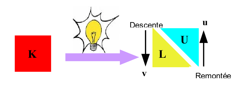
Once this breakdown is done, solving the problem is greatly facilitated. It is now only expressed in the form of the simplest linear resolutions that exist: based on triangular or diagonal matrices. These are the famous « downhill lifts » (”forward/backward algorithms”). For example in the case of a factorization \(LU\), the system (1.1-1) will be solved by
\(\begin{array}{c}\text{Ku}=f\\ \text{PK}=\text{LU}\end{array}\rangle \Rightarrow \begin{array}{c}\text{Lv}=\text{Pf}(\text{descente})\\ \text{Uu}=v(\text{remontée})\end{array}\) (1.3-2)
In the first lower diagonal system (descent), the intermediate solution vector \(v\) is determined. The latter then serves as the second member of the upper diagonal system (ascent) of which the vector \(u\) that interests us is a solution.
This phase is inexpensive (in dense), of the order of \({N}^{2}\) against \({N}^{3}\) for factorization [14] _ with \(N\) the size of the problem) and can therefore be repeated numerous times while keeping the same factorized. This is very useful when solving a problem such as multiple second members or when you want to perform simultaneous resolutions.
In the first scenario, the matrix \(K\) is fixed and the second member \({f}_{i}\) is successively changed to calculate as many solutions \({u}_{i}\) (the resolutions are interdependent). This makes it possible to pool and therefore amortize this initial cost of factorization. This strategy is widely used, especially in Code_Aster: non-linear loop with periodic updating (or no updating) of the tangent matrix (e.g. Aste r STAT_NON_LINE operator), subspace or inverse power methods (without Rayleigh acceleration) in modal calculation (CALC_MODES) in modal calculation (), thermo-mechanical chaining with material characteristics independent of temperature (MECA_STATIQUE),…
In the second scenario, we know all the \({f}_{i}\) at the same time and we organize, by blocks, the descent-ascent phases, to simultaneously calculate the independent \({u}_{i}\) solutions. It is thus possible to use more efficient high-level linear algebra routines, or even to play on memory consumption by storing the vector \({f}_{i}\) in an empty state. This strategy is (partially) used in*Code_Aster*, for example, in the construction of Schur complements of touch-friction algorithms or for substructuring.
Note:
Product MUMPS provides for these two types of strategies and even offers features to facilitate the construction and resolution of Schur complements.
Now let’s look at the factorization process itselves. It is already clearly explained in the other theoretical documentation of Code_Aster on the subject [R6.02.01] [R6.02.02], as well as in the bibliographical references already cited [Duf06] [Gol96] [Gol96] [Las98]. So we will not detail it. Let’s just specify that it is an iterative process organized schematically around three loops: one « called in \(i\) » (on the rows of the work matrix), the second « in \(j\) » (resp. columns) and the third « in \(k\) » (resp. factorization steps). They iteratively build a new \({\tilde{A}}_{k+1}\) matrix from some data from the previous one, \({\tilde{A}}_{k}\), via the classical factorization formula which is formally written:
\(\begin{array}{c}\text{Boucles en}i,j,k\\ {\tilde{A}}_{k+1}(i,j):={\tilde{A}}_{k}(i,j)-\frac{{\tilde{A}}_{k}(i,k){\tilde{A}}_{k}(k,j)}{{\tilde{A}}_{k}(k,k)}\end{array}\) (1.3-3)
Initially the process is activated with \({\tilde{A}}_{0}=K\) and at the last step, we recover in the square matrix \({\tilde{A}}_{N}\) the parts that are triangular (\(L\) and/or \(U\)) or even diagonal (\(D\)) that interest us. For example, in case \(LD{L}^{T}\):
\(\begin{array}{c}\text{Boucles en}i,j\\ \text{si}i<j:L(i,j)={\tilde{A}}_{N}(i,j)\\ \text{si}i=j:D(i,j)={\tilde{A}}_{N}(i,j)\end{array}\) (1.3-4)
Note:
The formula (1.4-3) contains the seed of the problems inherent in direct methods: in empty storage, the fact that the term \({\tilde{A}}_{k+1}(i,j)\) can become non-zero while \({\tilde{A}}_{k}(i,j)\) is (concept of filling in the factored, “fill-in”, therefore involving renumbering or “ordering”); the propagation of rounding errors or the division by zero via the term \({\tilde{A}}_{k}(k,k)\) (concept of pivoting and balancing the terms of the matrix or “scaling”) .
1.4. Direct methods: the different approaches#
The order of loops \(i,j\) and \(k\) is not fixed. You can switch them and perform the same operations but in a different order. This thus defines six variants \(\mathrm{kij},\mathrm{kji},\mathrm{ikj}\dots\) that will manipulate different areas of the current matrix \({\tilde{A}}_{k}\): « zone of the new calculated terms » via (1.3-2), « zone already calculated and used » in (1.3-2), « zone already calculated and unused », « zone already calculated and unused » and « zone not yet calculated ». For example, in variant \(\mathrm{jik}\), we have the following operating diagram for \(j\) fixed
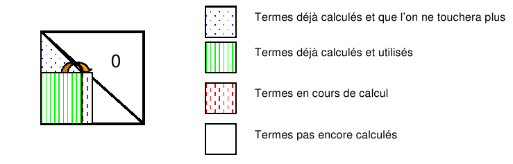
Figure 1.4-1._ Diagram for constructing a factorization « \(\mathrm{jik}\) » (“right looking”).
Notes:
The \(LD{L}^{T}\) method of Code_Aster (SOLVEUR/METHODE =” LDLT “) is a « :math:`mathrm{ijk}` » factorization, are the multifrontals of C.Rose (… =” MULT_FRONT”) and MUMPS (… =” “) and (… =” MUMPS”) oriented columns ( »:math:`mathrm{kji}` ») . *
Some variants have particular names: Crout algorithm ( » \(\mathrm{jki}\) « ) and Doolitle’s algorithm ( » \(\mathrm{ikj}\) « ) .
In the papers we often use Anglo-Saxon terminology designating the orientation of matrix manipulations rather than the order of the loops: “looking forward method”, “looking backward method”, “up-looking”, “left-looking”, “left-looking”, “”right-looking”, “left-right-looking”…
All these variants are still available as follows:
Whether we exploit certain properties of the matrix (symmetry, definition-positivity, band…) or that we are looking for the broadest scope of use;
Whether scalar or block treatments are performed;
That the decomposition into blocks is determined by memory aspects (cf. method :math:`LD{L}^{T}` paginated by*Code_Aster) or rather linked to the independence of subsequent tasks (via a multifrontal cf elimination graph [R6.06.02] §1.3);
That we reintroduce null terms into the blocks to facilitate access to data [15] _
and elicit very efficient algebraic operations, often*via* BLAS3 [16] _ (cf. multifrontal by C.Rose and MUMPS);
Whether the contributions affecting a block of rows/columns are grouped (“fan-in” approach, cf. pastiX) or whether they are applied as soon as possible (“fan-out”);
That in parallel, we seek to create different levels of sequences of independent tasks, whether we order them statically or dynamically, that we recover from calculation through communication…
Whether we apply pre and post-treatments to reduce filling and improve the quality of the results: renumbering the unknowns, scaling the terms of the matrix, partial (row) or total (row and column) pivoting, scalar or by diagonal blocks, iterative refinement…
To group them together, we often distinguish four categories:
The**classical algorithms*: Gauss, Crout, Crout, Cholesky, Markowitz (Matlab, Mathematica, Y12M…);
frontal methods (MA62…);
multifrontal methods (MULT_FRONT Aster, MUMPS,, SPOOLES, TAUCS, UFMPACK, WSMP…)
1.5. Direct methods: the main steps#
When treating sparse systems, the numerical factorization phase (1.3-3) does not apply directly to the initial matrix \(K\), but to a working matrix \({K}_{\mathrm{travail}}\) resulting from a preprocessing phase. And this in order to reduce filling, to improve the accuracy of the calculations and therefore to optimize subsequent costs in CPU and in memory. Roughly speaking, this working matrix can be written in the form of the following matrix product:
\({\mathrm{K}}_{\text{travail}}\mathrm{:}\mathrm{=}{\mathrm{P}}_{o}{\mathrm{D}}_{r}\mathrm{K}{\mathrm{Q}}_{c}{\mathrm{D}}_{c}{\mathrm{P}}_{o}^{T}\) (1.5-1)
the various elements of which we will describe later. We can thus break down the operation of a direct solver into four steps:
Pretreatments and symbolic factorization: it interchanges the order of the columns in the work matrix (via a permutation matrix \({Q}_{c}\)) in order to avoid divisions by zero of the term \({\tilde{A}}_{k}(k,k)\) and to reduce filling. In addition, it rebalances the terms in order to limit rounding errors (via scaling matrices \({D}_{r}/{D}_{c}\)). This phase can also be crucial for algorithmic efficiency (gain of a factor of 10 sometimes observed) and the quality of results (gain of 4 or 5 decimals).
In this phase, the storage structures for the hollow factored matrix and the auxiliaries (dynamic pivoting, communication…) required by the following phases are also created. In addition, the dependency tree of the tasks, their initial distribution according to the processors and the total expected memory consumption are estimated.
The renumeration step: it inverts the order of the unknowns of the matrix (via the permutation matrix \({P}_{o}\)) in order to reduce the filling involved in factorization. In fact, in the formula (1.3-3) we see that the factored term (\({\tilde{A}}_{k+1}(i,j)\ne 0\)) can contain a new non-zero term in its profile while the initial matrix did not include one (\({\tilde{A}}_{k}(i,j)=0\)). Because of the term \(\frac{{\tilde{A}}_{k}(i,k){\tilde{A}}_{k}(k,j)}{{\tilde{A}}_{k}(k,k)}\) not necessarily void. In particular, it is non-zero when non-zero terms from the initial matrix of the type \({\tilde{A}}_{k}(i,l)\text{ou}{\tilde{A}}_{k}(l,j)(l<i\text{et}l<j)\) can be found. This phenomenon can lead to very significant additional memory and calculation costs (the factored one can be 100 times bigger than the initial sparse matrix!).
Hence the idea of renumbering the unknowns (and therefore of permuting the rows and columns of \(K\)) in order to curb this phenomenon, which is the real « Achilles heel » of directs. To do this, we often use external products ((PAR) METIS, (PT) SCOTCH, CHACO, JOSTLE, PARTY…) or embedded heuristics with solvers (AMD, RCMK…). Of course, these products have different performances depending on the matrices processed, the number of processors… Among them, METIS and SCOTCH are very common and « often stand out » (gain up to 50%) ** (gain up to 50%).
The numerical factorization phase: it uses the formula (1.3-3) via the methods described in paragraph §1.4 above. This is by far the most costly phase that will explicitly build sparse factorizations \(L{L}^{T},LD{L}^{T}\) or \(LU\).
The resolution phase: it carries out the descents and ascents (1.3-2) from which « sprouts » (finally!) solution \(u\). It is incost and possibly pools subsequent numerical factorization (multiple second members, simultaneous resolutions, computation restart…).
Notes:
Steps 1 and 2 only require knowledge of the connectivity and the graph of the initial matrix. So finally only data that can be stored and manipulated in the form of integers. Only the last two steps use real numbers on the effective terms of the matrix. They only need the terms of the matrix if the scaling steps are activated (calculation of \({D}_{r}/{D}_{c}\) ) .
Steps 1 and 4 are independent while steps 1, 2 and 3, on the other hand, are linked. Depending on the products/algorithmic approaches, they are grouped differently: 1 and 2 are linked in MUMPS, 1 and 3 in SuperLu and 1, 2 and 3 in UFMPACK… MUMPS makes it possible to carry out steps 1+2, 3 and 4 separately but successively, steps 1+2, 3 and 4, or even to pool their results to perform various sequences. For now, in Code_Aster, we alternate the sequences 1+2+3 and 4, 4, 4… and again 1+2+… (cf. next chapter) .
Some products offer to test several strategies in one or more stages and choose the most suitable one: SPOOLES and WSMP for stage 1, TAUCS for stage 3 etc.
The renumbering tools of the first phase are based on very varied concepts: engineering methods, geometric or optimization techniques, graph theory, spectral theory, taboo methods, evolutionary algorithms, memetic algorithms, memetic ones, those based on so-called « ant colonies », those based on so-called « ant colonies », neural networks… Any chance is allowed to improve the local optimum in the form of which the renumber problem is expressed. These tools are also often used to partition/distribute meshes (cf. [:external:ref:`R6.01.03 <R6.01.03>`]*§6). For now, Code_Aster is using the renumbers METIS /AM/ AMD (for METHODE =” MULT_FRONT “and” MUMPS “), AMF/QAMD/PORD (for” MUMPS “), and RCMK [] _ 17 (for “ GCPC “,” LDLT “, and “ PESTC”) .
Whatever the linear solver [18] _
used, Code_Aster performs a preliminary factorization phase (step 0) to describe the unknowns of the problem (physical or late degree of freedom link/matrix row number via the data structure NUME_DDL ) and predict the ad hoc storage of the MORSE profile of the matrix.
1.6. Direct methods: the difficulties#
Among the difficulties that « empty direct methods » must overcome are:
The**manipulation of complex data structures* that optimize storage (cf. matrix profile) but that complicates the algorithm (cf. pivoting, OOC…). This contributes to lowering the « calculation/data access » ratio.
Effective data management with respect to the memory hierarchy and the IC flip-flop/ OOC [19] _
. This is a recurring question with a lot of problems, but it is important here because of the high computing power.
The management of the**hollow/dense trade* (for methods by fronts) with respect to memory consumption, ease of access to data and the efficiency of elementary building blocks of linear algebra.
Choosing the**right renumbering*: it’s an NP-complete problem! For large problems, the optimal renumbering cannot be found in a « reasonable » time. We must be content with a « local » solution.
Effective management of**propagation of rounding errors scaling, pivoting, and error calculations on the solution (direct/inverse error) [20] _ and packaging).
The**size of the factorized one that is often « bottleneck » No. 1*. Its distribution between processors (via distributed parallelism) and/or OOC do not always make it possible to overcome this pitfall (cf. figure 1.6-1).
Figure 1.6-1._ The « bottleneck » of sparse direct solvers: the size of the factored one.
This figure includes two examples: a canonical test case (cube) and an industrial study (pump RIS). With the following notations: \(\text{M}\) for millions of terms, \(\text{N}\) the size of the problem, the size of the problem, \(\text{nnz}\) the number of non-zero terms in the matrix, and \({K}^{\text{-1}}\) that of its factored renumbered*via* METIS. The superfactor when going from one to the other is noted in brackets.